1. Reversibility, irreversibility, and the arrow of time
Joule—Gay-Lussac expansion was introduced in Lesson 5. Recall that it is the expansion of a gas into a vacuum. The gas is initially confined to a region of volume inside a rigid, adiabatic vessel that is otherwise empty and has total volume . When the partition confining it is removed, the gas spreads spontaneously throughout the vessel and a new equilibrium is established.
This process is not only allowed by the first law; its energy balance is actually trivial. As we have seen, no work is done against a vacuum during the expansion, so , and the walls are adiabatic, so . The first law concludes that
Consequently, this energy balance does not forbid the reverse process. Yet everyday experience tells us that it never occurs on our scale: we do not see the air in a room spontaneously gather in one corner, leaving the rest empty. Many other phenomena of this kind are extremely common. An egg that has been cooked (even very slowly) does not become raw again on its own. Heat flows spontaneously from hot bodies to cold ones, never the other way round, and so on.
These observations reveal a particular, preferred direction in the thermodynamic evolution of a system, which the first law alone does not capture. To arrive at the second law, let us first ask whether the reverse process is possible. When it is, the original process is called reversible; otherwise, it is called irreversible.
Is Joule—Gay-Lussac expansion reversible? In everyday language, this might be taken to mean that the gas can be returned to its initial state. In that case, the answer is obviously yes. We need only compress the gas to volume , wait for it to recover its initial temperature, then put the partition back. However, it is crucial to understand that this reverses the process from the system's point of view alone; it does not constitute the reverse of the expansion for the whole “Universe”, meaning the system and its surroundings.
Indeed, to compress the gas, assumed ideal here, the surroundings must supply work to it. If the compression is performed at constant temperature, say, the gas releases this energy as heat. At the end of the operation, the gas has returned to its initial state, but the surroundings have supplied work and received heat in compensation: restoring the system has changed the state of the outside world.
The distinction is subtle but essential. When we decide to reverse an irreversible process, the system itself has lost the memory of having undergone the process , since it has returned to state , but the surroundings retain a trace, or, if we wish, a memory of it. Schematically:
with . What characterizes an irreversible process is that it cannot be completely erased. Any attempt to erase this trace in the surroundings can only transfer it to another system, and so on.
A physical memory is nothing other than a trace of a past event present in a system. All recording devices are physical systems whose present state depends on what happened earlier. Even our own memory rests on a particular state of our brain, correlated with a previous event. The future state carries a memory of the past state, whereas the past state carries no memory of the future state. In other words, the arrow of time and the possibility of forming memories seem to refer to the same thing.1
It is in this precise sense that thermodynamics, by modelling irreversible processes that cannot be erased, introduces what is called the thermodynamic arrow of time.
Of course, attentive readers will have noticed that we have not proved that expansion into a vacuum is irreversible. We have shown that one particular attempt to restore the system and its surroundings fails. Claiming that this holds for every conceivable process is a much stronger universal statement, requiring new tools to establish it. This will be the role of the second law of thermodynamics. It introduces entropy, a new quantity capable of showing that a change has occurred somewhere and cannot be erased without being displaced elsewhere.
2. Reversible processes
To arrive at the second law, let us now introduce, as a counterpart, a particular class of thermodynamic processes. The following definition summarizes what we have just said.
If no return process allows this complete restoration, the initial process is called globally irreversible.
The initial and final states of the system alone are therefore insufficient to decide reversibility: the changes produced in its surroundings must also be known.
This definition is global. It concerns the outcome of the process for the system and everything that took part in it, but does not specify the path followed. It asks only whether every trace of the process can be erased. In particular, it does not require the return process to follow exactly the original path in reverse.
The definition adopted here differs from that in most textbooks. This is also why we add the adjective “global”. Standard presentations often bring together two distinct ideas under the same term: restoring the system and its surroundings, on the one hand, and being able to follow the same path in reverse, on the other. This is the case, for instance, in the textbook by Çengel and Boles [5]. Other presentations emphasize the second characterization, as in the textbook by Atkins and de Paula [6]. We nevertheless consider it important to distinguish them clearly. An approach similar in spirit to ours, although different, is proposed by Lieb and Yngvason [7] in their axiomatic reconstruction of thermodynamics.
We therefore introduce the following complementary definition.
The initial path can then be retraced: each infinitesimal step can be reversed, and the reversed steps joined together in the opposite order. Thus, if the forward process follows the sequence
the reverse process can follow exactly the same sequence in the other direction. The thermal and mechanical exchanges then change sign at every step. The reverse process is, so to speak, a film of the initial process played backwards.
Local reversibility implies global reversibility by construction. The converse does not hold a priori, since a global restoration could follow another path. Expansion into a vacuum is not quasi-static, so it cannot be locally reversible, but this does not yet prove that it is globally irreversible.
Why introduce this distinction, which is not always made explicitly in thermodynamics courses? Because experience shows that reversibility is an extremely difficult concept for beginners. In particular, confusing the global and local intuitions creates a major difficulty: students are too often led to confuse the definition of reversibility with the physical conditions for reversibility, i.e. the operational assumptions that allow a real thermodynamic process to be regarded as reversible.
Let us examine these conditions. First, slowness alone is insufficient. Heat transfer can be made as slow as desired by inserting a very poorly conducting wall between two bodies. As long as their temperatures differ by a finite amount, the heat transfer remains irreversible.
Being quasi-static, though necessary for local reversibility, is insufficient too. Consider a gas compressed very slowly by a piston subject to friction. The gas may remain arbitrarily close to mechanical equilibrium at every instant. Yet part of the work supplied is converted into heat by friction. When the gas is subsequently returned to its initial state, this heat remains somewhere in the surroundings: the process has left a trace.
Friction is only one of many causes of irreversibility. This is why one often speaks of a “quasi-static process without dissipation”. Used in a broad sense, this expression means that the system passes through a succession of equilibrium states and that the process is driven by infinitesimal differences in pressure, temperature or chemical potential, without friction, viscosity or hysteresis. In the usual framework of thermodynamics, these conditions allow a locally reversible process to be constructed. They are conditions for its realization, not the general definition of reversibility.
The locally reversible processes constructed in this way are ideal limits. A real process can approach them as closely as experimental devices allow, but any finite difference in pressure, temperature or chemical potential, as well as any dissipative phenomenon, produces residual irreversibility.
3. Towards a new state function
The other advantage of the global definition of reversibility is that it reveals both a structural difficulty and the way it can be resolved.
The difficulty is as follows. To show that a process is reversible, it suffices to find a return process that completely restores the system and its surroundings. To show that it is irreversible, one must establish that no such process exists, which is much harder.
This suggests a solution. The global definition does not ask how the return must occur; it concerns only the possibility of connecting the initial and final states of the complete system . It would therefore be particularly useful to have a state function whose change has a prescribed sign for every possible process. Such a function would immediately tell us whether the reverse process is possible. Suppose we have an additive state function satisfying the following criterion for every possible process:
We would then have:
In particular, if a process produces , a process restoring the initial state of the complete system would have to produce the opposite change, since is a state function. We would thus have , showing that this return process is impossible. Section 9 will establish the other implications and thereby justify the entire characterization announced above. This is how the second law of thermodynamics will work. The quantity is called entropy. The non-decrease of total entropy is the entropy formulation of the second law.
There are two possible routes to constructing the theory. The first directly postulates the existence of entropy and its increase principle, then uses this quantity to characterize reversible and irreversible processes. This postulatory approach is particularly well developed in Callen's book [8]. The second, more historical route starts with heat engines and leads to the theorems of Carnot and Clausius, then to entropy. This is the route we follow here.
4. The second law: operational statements
Throughout the following discussion of thermal machines, the working fluid is a closed system: it exchanges no matter with its surroundings. It undergoes a closed cycle, meaning that it returns to its initial thermodynamic state at the end of every cycle. Its internal energy change over a cycle is therefore zero, , even though it has exchanged heat and work with its surroundings.
We began this lesson by observing that heat flows spontaneously from hot to cold, never the other way round. In 1850, Clausius elevated this observation to a more general principle: it is impossible to place between a hot and a cold reservoir a thermodynamic system whose sole effect would be to reverse this spontaneous transfer.
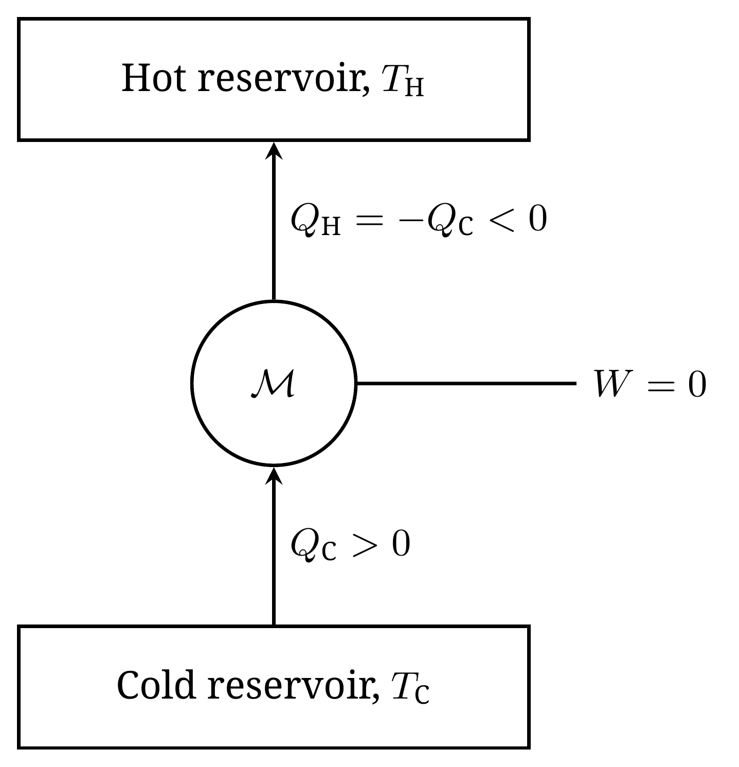
The words sole effect are essential. A refrigerator does transfer heat from cold to hot, but must receive work from its surroundings to do so. This statement cannot be deduced from the first law. It is a new physical principle, which we will show to be equivalent to the existence of entropy and its properties. For this construction, we will need another formulation, proposed by Kelvin in 1851 and subsequently refined by Planck.
We already encountered this statement in the first lesson. It forbids the existence of a perfect air conditioner that would cool your apartment by extracting heat from it and converting all this thermal energy into useful work.
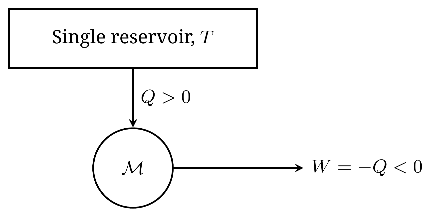
These two statements are related by the following theorem.
Proof.
When the two machines are combined, their work transfers cancel. The net heat received by the combination from the hot reservoir is therefore
The sole effect of the combination is to extract heat from the cold reservoir and deliver it to the hot reservoir. The Clausius statement is violated.
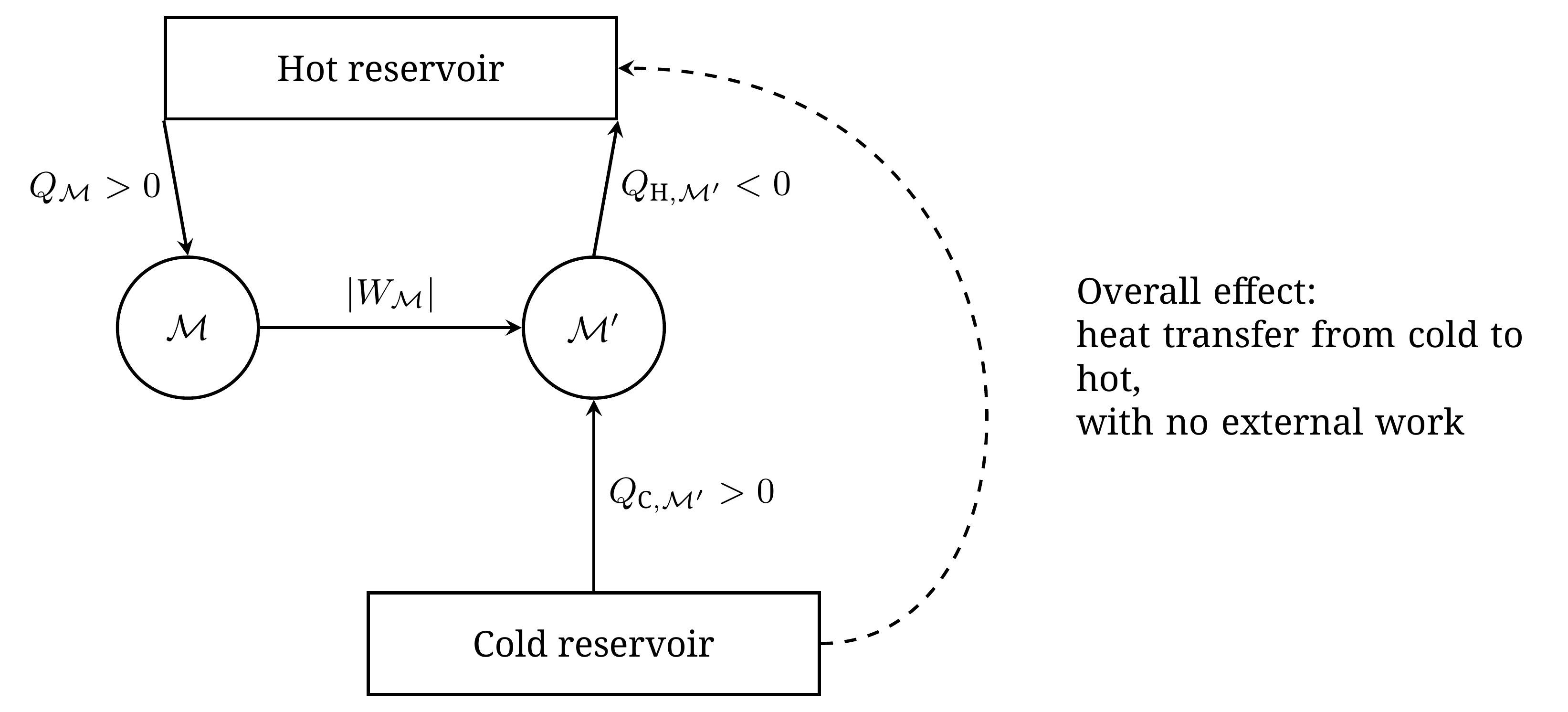
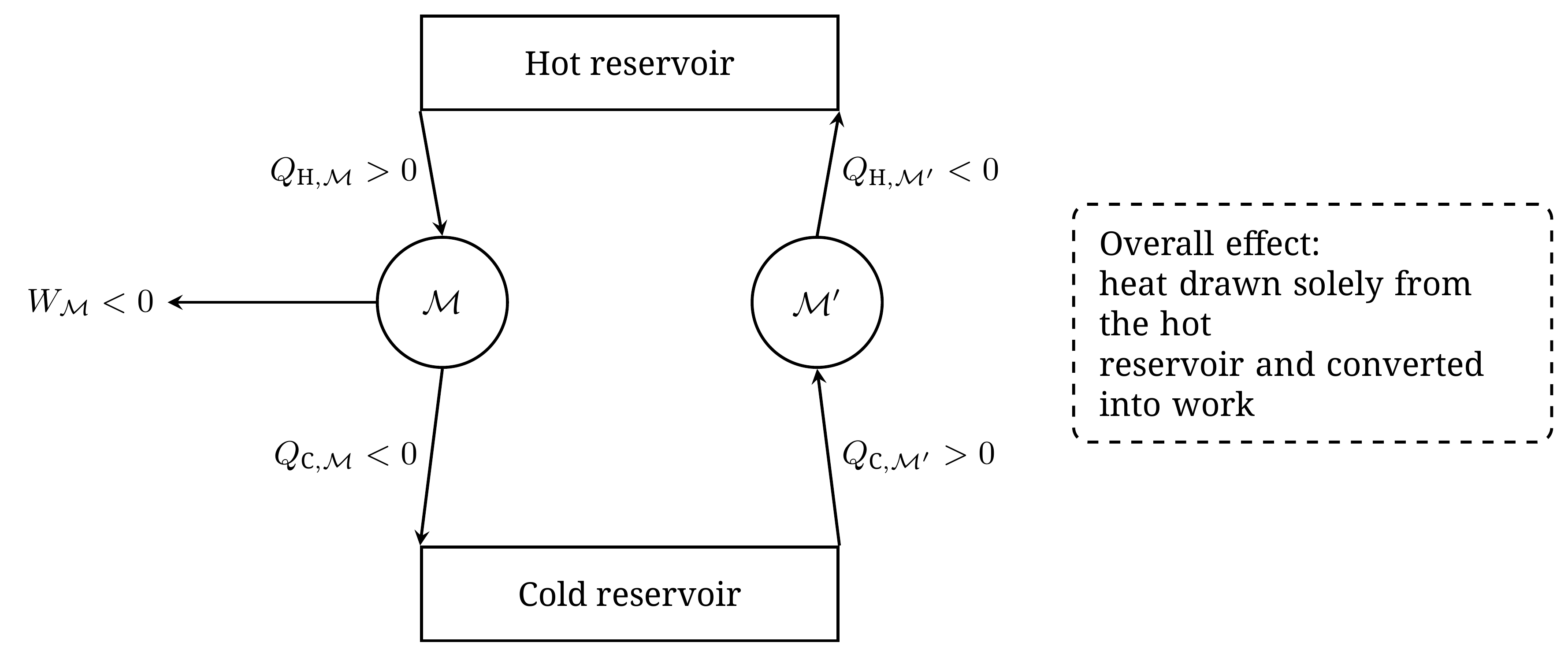
Conversely, suppose that Clausius's statement is false. There would exist a machine capable of extracting heat from the cold reservoir and delivering the same amount to the hot reservoir without receiving work. Let us couple it to an ordinary engine operating between the same reservoirs. The machines are adjusted so that the heat rejected to the cold reservoir by the engine is exactly extracted by :
The net exchange with the cold reservoir vanishes. The first law then shows that the net heat extracted from the hot reservoir equals the magnitude of the work supplied by the engine. The combination would thus convert heat extracted from a single reservoir into work. Kelvin's statement would be violated.
These statements will allow us to establish Carnot's theorems on the efficiency of heat engines, then the Clausius inequality, from which we will construct entropy.
5. Carnot's theorems
In the first lesson, we presented thermodynamics as a theory born from the search for more efficient heat engines. The central question was whether there is a fundamental limit to engine efficiency, independent of the particular technical difficulties of construction. We can now answer this question precisely. The following proofs may be skipped on a first reading: initially, it is more important to understand the sequence Carnot's theorems Clausius inequality construction of entropy. The proofs can be revisited later.
First consider two-reservoir machines, operating between only two thermal reservoirs: a hot reservoir at temperature and a cold reservoir at temperature . When operating as an engine, the machine receives heat from the hot reservoir and heat from the cold reservoir. In other words, it rejects the amount of heat to the cold reservoir. It also receives work , meaning that it supplies work to its surroundings. The first law requires .
To compare how effectively these engines operate, let us introduce their efficiency.
5.1. Maximum efficiency
and if the cycle of is globally irreversible, the inequality is strict: .
Proof.
In other words, for the same work, the supposedly more efficient engine extracts less heat from the hot reservoir than the reverse cycle of returns to it. The hot reservoir therefore receives a net amount of heat. The work transfers of the two machines cancel, and both working fluids return to their initial states. By energy conservation, the heat received by the hot reservoir has been extracted entirely from the cold reservoir. The sole effect of the combination would be heat transfer from cold to hot without any work input. This contradicts Clausius's statement.
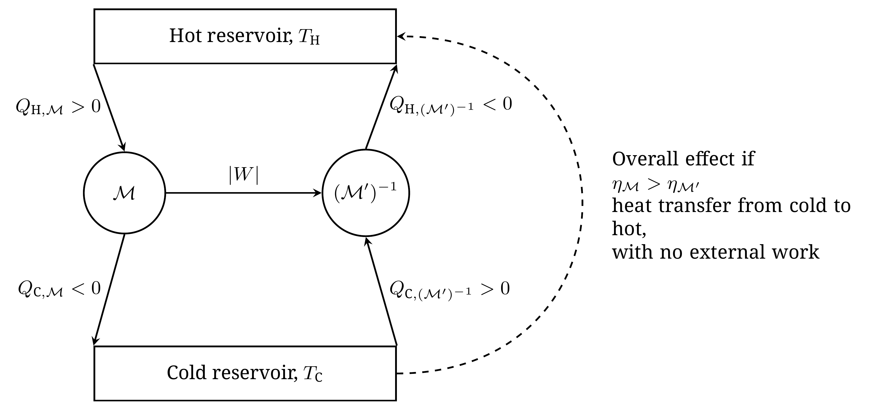
The initial assumption is therefore impossible, and .
Now consider equality: . Keeping the same coupling and adjustment of the machines, their work and heat exchanges now cancel exactly. This means that the cycle of is globally reversible. To understand this, imagine the two operations taking place one after the other. First run as an engine: it returns to its initial state, but the two reservoirs and the work source have changed. Then leave at rest and run in reverse, supplying it with the work previously collected. This second operation exactly cancels the changes in the two reservoirs and the work source. The auxiliary machine also returns to its initial state, since it completes a cycle. At the end of these two operations, the system and all its surroundings, including the auxiliary machine, have thus returned to their initial states. This is precisely the return required by the definition of global reversibility. Equality of the efficiencies therefore implies that the cycle of is globally reversible. By contraposition, if this cycle is globally irreversible, equality is excluded and . This argument does not, however, prove that the cycle of is locally reversible. We have erased its effects on the surroundings using another machine, without making retrace its own states in reverse. With the definitions adopted in this lesson, the strict inequality is therefore established for a globally irreversible cycle. The mere fact that a cycle is not locally reversible is insufficient, at this stage, to conclude that its efficiency is strictly lower.Proof.
Remark: the absolute temperature scale.
The second theorem makes the ratio of a locally reversible machine universal. It thus allows an absolute temperature independent of the working fluid to be defined: the Kelvin scale (see Section 11.1 for details).
To calculate the universal efficiency, it suffices to calculate it in one particular case.
5.2. The Carnot cycle of an ideal gas
This cycle uses an ideal gas and consists of two isothermal processes joined by two adiabatic processes, all locally reversible. Denote its four vertices by , , and :
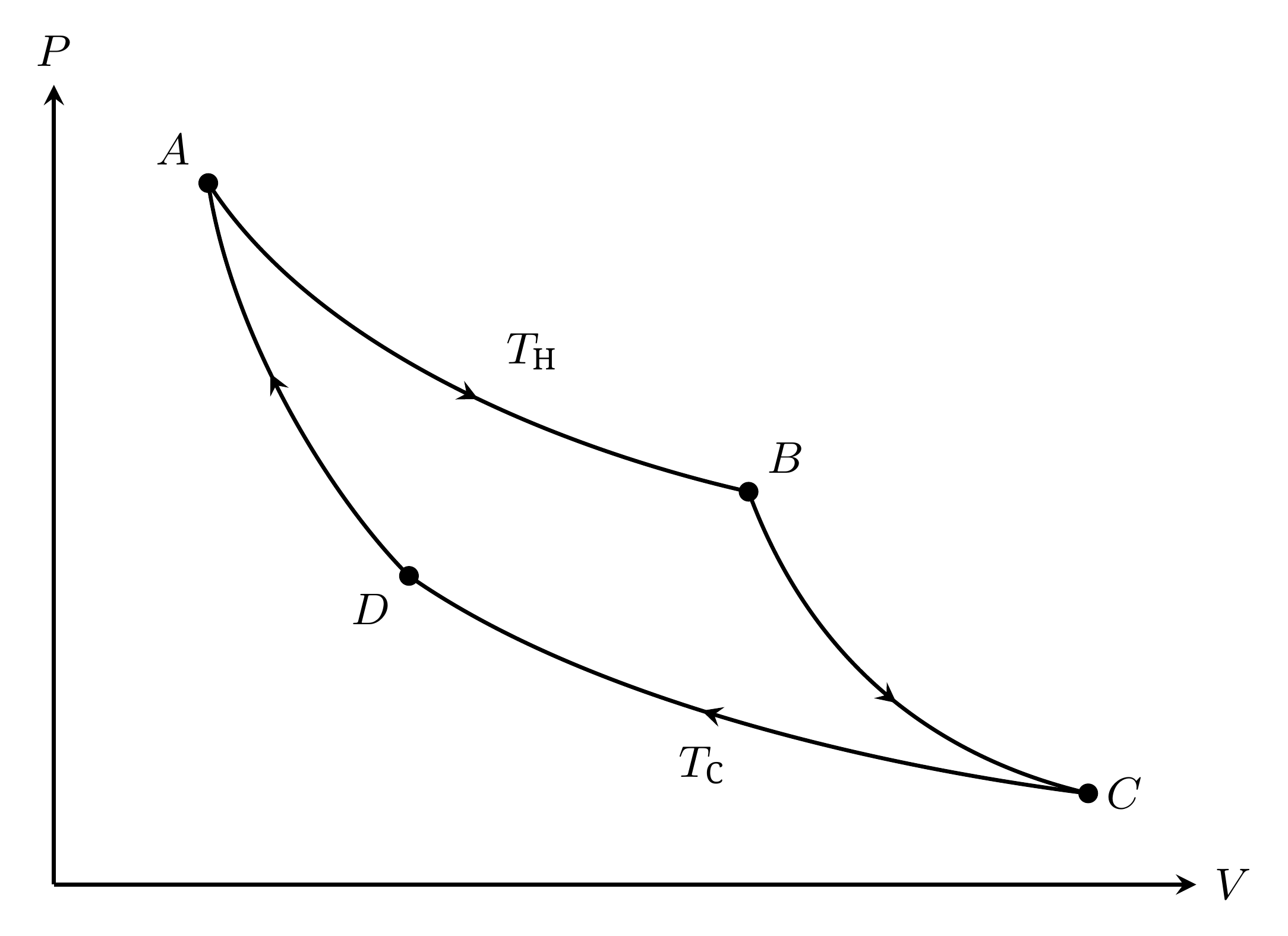
Proof.
During the isothermal compression , we similarly obtain
The amount of heat rejected to the cold reservoir is therefore .
Laplace's law , seen in Lesson 5, applied to the two adiabats givesDividing these equalities gives . The logarithms in the two isothermal exchanges are therefore equal, hence
The efficiency of the Carnot cycle is thus
which completes the proof.
6. The Clausius inequality
Carnot's theorems set a limit on the efficiency of two-reservoir engines. We will now deduce a constraint on heat exchanges over a cycle, the Clausius inequality, which will lead us to introduce entropy. For an arbitrary two-reservoir engine, Carnot's first theorem gives
It follows that
and since ,
This is the Clausius inequality for a two-reservoir machine. It generalizes to any finite number of thermal reservoirs:
Equality holds for a locally reversible cycle. The inequality is strict for a globally irreversible cycle.
Its proof is given in Section 11.2.
7. Constructing entropy
Now suppose that the external temperature at which the machine exchanges heat varies continuously during the cycle. We idealize these exchanges by a continuous family of reservoirs and assume that we can take the limit of the result established for finitely many reservoirs. The cycle can be divided into portions small enough for each exchange to occur at an almost constant external temperature. In the continuous limit, the sum becomes an integral over a complete cycle:
Here the circle in the symbol reminds us that the system returns to its initial state. If the cycle is locally reversible, the system passes through a succession of equilibrium states and has a temperature at every instant that differs only infinitesimally from the external temperature. In this case, we may identify and obtain, for any locally reversible cycle:
Be sure to distinguish these two formulas: the first concerns an arbitrary cycle, with the heat actually exchanged and the external temperature . The second concerns a locally reversible cycle: denotes the heat exchanged along this path, and the system's temperature, equal to in the reversible limit.
This equality holds for every locally reversible cycle. Let us show that it implies path independence and thus allows us to define a state function. Let and be two equilibrium states of the system, and and two locally reversible paths joining them. Following , then in reverse, forms a locally reversible cycle. The preceding equality then gives
The integral of between and therefore does not depend on the locally reversible path chosen. It depends only on the initial and final states. The differential form is thus exact on the domain considered: it is the differential of a state function, which we call entropy. We obtain:
In differential form, along a locally reversible path, we have
The subscript “rev” on the exchanged heat is crucial. It would be wrong to write for any heat received by an arbitrary system. This is true only if the transfer is reversible.
8. Properties of entropy
Unit
The preceding equations fix the unit of entropy: it is expressed in joules per kelvin.
Additivity and extensivity
As for energy in Lesson 4, we consider macroscopic systems whose mutual interactions are negligible. This is a good approximation for systems with short-range interactions. In this framework, we assume the following additivity property.
Within the same framework, we assume that entropy is also extensive, in the sense of Lesson 3: multiplying the size of the system by , while keeping its intensive variables fixed, multiplies its entropy by :
For systems with long-range interactions, additivity and extensivity are no longer guaranteed. We will return to these subtle issues in the more advanced part of this book.
Entropy, energy and temperature
Consider a simple, closed system of fixed composition subject only to pressure work. The number of particles therefore remains constant. Along a quasi-static process, the first law reads
If the process is also locally reversible, we obtain
or
This equation is called the fundamental relation. Although obtained for a locally reversible process, it holds for any elementary process connecting two equilibrium states, since and are state functions. We will study it in detail in the next lesson. For now, the properties of differentials give
The reciprocal temperature therefore measures the change of entropy with internal energy, at fixed volume and amount of substance. In this lesson, we consider states with absolute temperature . The preceding relation then shows that entropy is an increasing function of .
9. The quantitative formulation of the second law
We now have all the tools needed to give the second law its usual entropy formulation. We present it as three successive theorems; these are indeed theorems and not principles, since we adopted the Clausius statement as our principle.
In what follows, it is important to specify which whole the entropy refers to. We denote the entropy of the system under study by , and that of the system and its surroundings by . The first theorem concerns an isolated system. The second concerns the isolated combination . The third returns to the system alone, closed but able to exchange energy: its entropy may decrease even though total entropy does not.
To understand the scope of this statement, recall that an isolated system already at equilibrium does not evolve spontaneously. The statement becomes fully meaningful when the initial state is a constrained equilibrium, maintained, for example, by a partition that is subsequently removed without any exchange with the surroundings. The system then evolves towards a new equilibrium whose entropy is greater than or equal to that of the initial state. Joule expansion into a vacuum is one example.
The proof of this theorem is instructive because it shows how to use the Clausius inequality.
Proof.
By the definition of entropy, the second integral equals . We therefore obtain
If the system is isolated, no heat exchange occurs during the actual process : its contribution to the Clausius integral is zero, without any need to define . We thus recover .
If the system under study is not isolated, its entropy may decrease when it releases heat to its surroundings. Including all the bodies and devices involved in the process again gives an isolated whole. The preceding result, together with entropy additivity, then gives the formulation announced in Section 3:
When the surroundings consist of thermal reservoirs and an ideal work source, the following equivalences hold:
Proof.
The second law requires each to be non-negative. Both are therefore zero; in particular, .
Conversely, suppose the process satisfies . By the assumption of reversible connectedness, return the system from to along a locally reversible path. This return does not change total entropy: . Over the complete round trip, we therefore have . Since the system has returned to its initial state, ; the entropy change of the surroundings over this cycle is therefore zero as well. This does not mean that every reservoir has returned to its initial state: some may have released heat and others received it, with their entropy changes cancelling. The work source may also have changed. These exchanges still need to be cancelled. As in the proof of the Clausius inequality (Section 11.2), locally reversible auxiliary machines can be used to provide this compensation. They themselves complete cycles. The system and all its surroundings have then returned to their initial states: we have constructed a global return.A globally irreversible process therefore increases total entropy. To track the balance for the system alone, let us now distinguish two contributions: entropy exchanged with the surroundings and entropy produced. We define:
Since , releasing heat corresponds to releasing entropy. The entropy of the system may thus decrease if it releases more than it produces, as expressed by the following balance.
The quantity is called the entropy produced. It is non-negative.
If the entropy of the system is defined at every instant, the balance takes the differential formProof.
This decomposition into exchanged and produced entropy is notably the one used by Prigogine in his 1977 Nobel lecture [4]. You will encounter it in other courses. Note that only is the differential of a state function here; the terms and depend on the process, and are therefore inexact differentials, hence the notation (Prigogine writes and ).
10. Entropy, direction of evolution and equilibrium
The first law imposes energy conservation; the second specifies the direction of possible evolutions through the increase of total entropy. Let us now use this balance to quantify the irreversibility of Joule expansion and study the spontaneous direction of thermal or mechanical transfer. We will remain within the framework of closed systems, each time distinguishing the system under study from the isolated whole to which the second law applies.
10.1. Calculating an entropy change
The fundamental trick of thermodynamics is as follows: since is a state function, its change between two equilibrium states and of the system does not depend on the actual process followed. Even if that process is irreversible, we can imagine a locally reversible path joining the same states and calculate
The heat belongs to the path chosen for the calculation. It need not equal the heat actually exchanged during the process under study. Once has been calculated, we can return to the actual process to determine the exchanged and produced entropy.
10.2. The irreversibility of Joule expansion
Let us apply this method to Joule expansion into a vacuum. During the actual process, the ideal gas expands from volume to volume without receiving either heat or work. Its internal energy remains constant, so its final temperature equals its initial temperature. To calculate its entropy change, imagine a locally reversible isothermal expansion between the same states. The first law gives
since for an isothermal process of an ideal gas. Integrating along this path gives
During the actual expansion, no energy is exchanged with the surroundings. In the idealization adopted, the vessel remains unchanged and removing the partition itself leaves no external change. We therefore have , and the entropy balance for the isolated whole gives
Joule—Gay-Lussac expansion is therefore globally irreversible. The increase of total entropy shows that no procedure can restore the gas and its surroundings without leaving a trace elsewhere.
10.3. The irreversibility of heat transfer
Consider two closed systems and , at fixed volumes, placed in thermal contact. They need not be gases: the following reasoning is general. They exchange neither matter nor work, but may exchange heat. The combination is assumed isolated. A poorly conducting wall makes the exchanges slow enough for each system to remain close to internal equilibrium. Each then evolves quasi-statically and has a temperature at every instant. We neglect the wall's contributions to energy and entropy.
At fixed volume and amount of substance, the fundamental relation gives, with ,
Since the combination is isolated, the first law and energy additivity require
Denote by the signed heat received by system . Since neither system exchanges work,
Energy conservation therefore gives
Writing for the heat transferred from 1 to 2, counted positively in that direction, we thus have
By entropy additivity, the second law applied to the isolated whole gives
When , this inequality requires : heat therefore flows from hot to cold. If , its direction reverses and heat again flows from hot to cold. We thus see how the second law fixes the direction of possible exchanges, in agreement with everyday experience.
When , any nonzero transfer in the allowed direction gives . Spontaneous heat transfer from hot to cold is therefore globally irreversible, even if each part evolves quasi-statically.
10.4. Entropy and equilibrium
Let us continue the preceding example. If , heat transfer from hot to cold increases total entropy. Since the wall conducts heat, this transfer continues as long as a temperature difference remains. Thermal equilibrium therefore requires .
We then find that vanishes for any small redistribution of energy between the bodies: total entropy is stationary. This motivates the general criterion that we will assume: at equilibrium, the entropy of an isolated whole is stationary under small internal variations allowed by the constraints. In other words, its first-order change vanishes. This criterion provides a necessary condition for equilibrium; it proves neither uniqueness nor convergence of every evolution towards that state.
To illustrate this, consider a rigid, isolated cylinder containing two compartments of ideal gas separated by a movable, diathermal wall impermeable to matter. The wall moves without friction and is subject to no additional force. We neglect its own energy. Conservation of total energy gives , while conservation of total volume requires . The fundamental relation then gives
The wall allows both heat transfer and displacement: energy and volume redistributions can therefore be varied independently to test stationarity. Here we compare neighbouring states, rather than describing the wall's actual motion. At equilibrium, this change must vanish for all such variations. Both coefficients vanish: we obtain , then , hence
These familiar conditions show the usefulness of the stationarity criterion, but also the importance of constraints. If the wall remains movable but becomes adiabatic, it forbids heat transfer while allowing work exchange: and are then no longer independent variations. We therefore cannot set the two coefficients separately to zero as before. Mechanical equilibrium still requires , by force balance on the wall, but this condition is insufficient to impose .
11. Going further
11.1. Thermodynamic temperature
Kelvin's construction of an absolute temperature scale rests on Carnot's second theorem. Temporarily denote an empirical temperature, increasing from cold to hot, by . For a locally reversible two-reservoir machine between , let be the heat extracted from the hot reservoir and that rejected to the cold reservoir. The ratio
depends neither on the fluid nor on the cycle, since the efficiency is universal by this theorem. But this universality is not yet enough to write as a ratio : we must check that comparisons between reservoirs remain consistent when made through an intermediate reservoir.
Consider three reservoirs, with . Combine two locally reversible machines, one between reservoirs 1 and 2 and the other between 2 and 3. Adjust them so that the heat rejected to reservoir 2 by the first is exactly extracted by the second. The intermediate reservoir then undergoes no change. The combination constitutes a locally reversible machine between 1 and 3: both cycles and all their exchanges can be reversed. The universality of efficiency therefore requires
Reversing the cycle gives . Set and choose a reference reservoir , to which we assign a temperature . Then define
Each temperature is thus defined by comparison with the same reference. To express the ratio on this scale, apply the composition law:
We deduce
or
We thus recover, without using an ideal gas,
where the scale constructed in this way, through the ideal efficiencies of reversible machines, is the Kelvin scale.
11.2. Proof of the Clausius inequality
We prove here the Clausius inequality stated in Theorem 5.
Proof.
The relation obtained for a reversible machine gives2
hence
Each auxiliary machine also exchanges work
Its direction of operation depends on the signs of and . Thus, need not be hotter or colder than all the reservoirs.
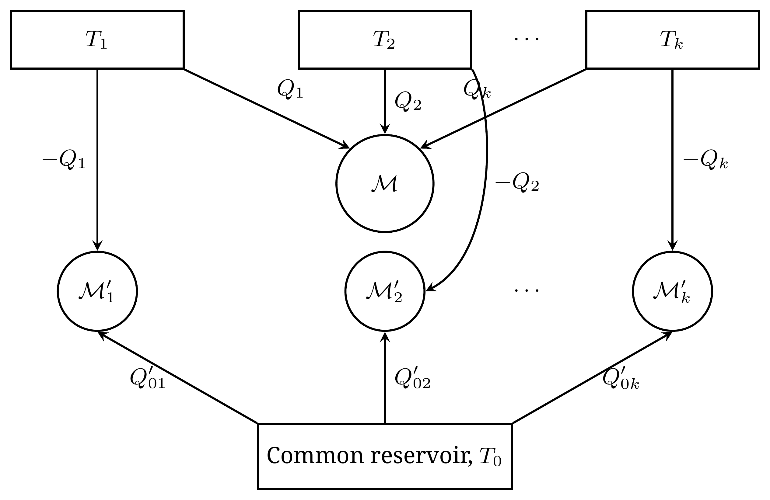
After combining all the machines, exchanges with each reservoir cancel. The only uncompensated heat exchange is with :
The composite machine is cyclic. The first law therefore requires
If were positive, the composite machine would extract heat from a single reservoir and convert it entirely into work. Kelvin's statement forbids this. We must therefore have . Since , the stated inequality follows.
If the cycle is locally reversible, it can run in reverse, and all exchanges change sign. Applying the Clausius inequality in both directions givesThe sum is therefore zero.
Conversely, if the sum is zero, the auxiliary machines restore all the reservoirs without changing reservoir and without producing net work. The work source also returns to its initial state: the weight returns to its initial height. Since the auxiliary machines themselves complete cycles, they construct a return that erases the external changes produced by the initial machine. The cycle is then globally reversible. Here, equality therefore characterizes global reversibility, without by itself proving local reversibility of the original path.11.3. A statistical interpretation of free expansion
In Lesson 4, we distinguished the macrostate, described by a few thermodynamic quantities, from the microstates, which specify the positions and velocities of the particles. The same macrostate is compatible with an immense number of microstates, indistinguishable on our scale. This distinction explains the irreversible character of free expansion.
Imagine an ideal gas of particles, initially confined to the left half of an isolated vessel, with the right half empty. Once the partition is removed, each particle has access to twice the volume. The number of accessible spatial configurations is thus multiplied by for each particle, or by for the gas as a whole. Configurations in which particles are distributed between the two halves are then far more numerous than those in which they are all on the left.
In thermodynamics, entropy changes are calculated along a locally reversible path between the equilibrium states considered. Statistical physics gives access to the entropy of an equilibrium state by counting microstates. Boltzmann's formula thus relates entropy to the number of microstates compatible with the macrostate:
Here, denotes this number of microstates, counted using the same convention, and is Boltzmann's constant, expressed in joules per kelvin. In our example, the energy of the gas remains unchanged, while doubling the volume multiplies by . The entropy increase is therefore
since , where is the amount of substance of the gas. We recover the thermodynamic result for an expansion from to .
This statistical interpretation explains why the spontaneous return of all particles to the left half, excluded by thermodynamics, is not strictly impossible. At equilibrium, each particle has probability of being in this half. Assuming their positions are independent, the probability that they are all there at a given instant is
For a macroscopic number of particles, this probability is astronomically small, and it is correct to regard it as zero in practice. Statistical physics thus shows that irreversibility is not an absolute phenomenon: it is probabilistic in nature.
11.4. The paradox of microscopic reversibility
How can irreversible evolution result from reversible microscopic laws? Recall that the laws of classical mechanics are time-reversible. This is Loschmidt's paradox: for every evolution in which entropy increases, these laws allow a reverse evolution in which it decreases. We therefore need to understand why the two directions of evolution, possible on the microscopic scale, are not observed equally often on our scale.
The macroscopic description of the system retains only part of the microscopic information. If all velocities could be reversed exactly after an expansion, the system would retrace its evolution. But replacing a partition or reversing the change in external pressure does not achieve this operation. These actions control only a small number of macroscopic variables and leave unchanged the microscopic details into which the information has dispersed.
This observation explains why reversibility of the microscopic laws does not make macroscopic processes reversible. Boltzmann entropy describes the macrostate to which the system belongs. An exact microscopic description, by contrast, retains far more information than the thermodynamic variables. In free expansion, the gas is initially prepared in a low-entropy state, whose evolution is very likely to lead to a state of higher entropy. The return would require very particular microscopic correlations, which exact reversal of the velocities would produce.
12. References
- Leonard Mlodinow and Todd A. Brun, Relation between the psychological and thermodynamic arrows of time, Physical Review E 89, 052102 (2014).
- David H. Wolpert and Jens Kipper, Memory Systems, the Epistemic Arrow of Time, and the Second Law, arXiv:2309.10927 (2023).
- Jerzy Gołosz, Does the Thermodynamic Arrow Explain the Psychological Arrow of Time?, Minds and Machines 35, 48 (2025).
- Ilya Prigogine, Time, Structure, and Fluctuations, Nobel Lecture, 8 December 1977; published in Science 201, 777—785 (1978). See p. 778, Entropy Production.
- Y. A. Çengel and M. A. Boles, Thermodynamics: An Engineering Approach, 8th ed., McGraw-Hill (2015), chap. 6, Reversible and Irreversible Processes.
- P. Atkins and J. de Paula, Atkins' Physical Chemistry, 9th ed., Oxford University Press (2010), chap. 2, The First Law.
- E. H. Lieb and J. Yngvason, The Physics and Mathematics of the Second Law of Thermodynamics, Physics Reports 310, 1—96 (1999).
- H. B. Callen, Thermodynamics and an Introduction to Thermostatistics, 2nd ed., Wiley (1985)