Application to the Ideal Gas

Until now, the first law has been formulated without assuming any particular model for the system. For a closed system whose macroscopic kinetic and potential energies do not change, it reads

$$\Delta U=Q+W.$$

However, this relation is not sufficient to calculate $\Delta U$, just as Newton's second law does not predict the evolution of a system until the forces acting on it are known. We must therefore further characterize the system under study: we will now do so for the ideal gas.

1. The equations of state of an ideal gas

A first equation of state of the ideal gas is

As we saw in Lesson 2, this relation is the result of a long history of experimental investigation. By itself, it tells us nothing about the internal energy of the gas. Other experiments are needed for that purpose. The following section, which may be skipped on a first reading, presents the experimental approach leading to the other key formula for an ideal gas:

where $c_V$ is a constant to which we will return and $U_0(n)$ is a reference term independent of temperature. Note at this stage that the thermodynamic formalism does not allow these equations of state to be derived. Statistical physics, however, will make it possible to recover them from a microscopic model.

1.1. Joule-Gay-Lussac expansion

The key experiment consists in observing the expansion of a gas into a vacuum. In practice, a sufficiently dilute gas is used to reduce interactions between molecules and thus approach the ideal-gas model. A rigid, thermally insulated vessel is divided into two compartments. The first contains the gas at equilibrium and the second is evacuated. The partition separating them is removed, a new equilibrium is allowed to establish itself, and the final state is then characterized experimentally.

Gay-Lussac was the first to perform this type of experiment at the beginning of the 19^th century; Joule repeated it later, around 1845. The important experimental result is that no change in the temperature of the gas is observed between the initial and final states. In reality, for a real gas, a small change remains and may be positive or negative depending on the gas and the conditions; it tends to zero, however, as the density decreases. In the ideal model, we are therefore led to consider that $T_B=T_A$ exactly.

To interpret this result, let us examine what the first law says. The gas expands into a vacuum, so the external pressure is zero and therefore $W=0$. Moreover, the walls of the system are thermally insulated, so $Q=0$ as well. The first law then requires

$$\Delta U=0.$$

Let us assume for the moment that the internal energy can be written as $U=U(T,V,n)$; this choice of variables will be justified after the second law has been established. Since the system is closed, $n$ is fixed. Repeated for different initial and final volumes, the experiment shows that at fixed temperature (since $T_B=T_A$), the internal energy does not change when the volume changes ($\Delta U=0$). It follows that

This property constitutes Joule's law: the internal energy of an ideal gas does not depend on its volume. This experiment does not yet determine the form of the function $U(T,n)$.

1.2. Internal energy of an ideal gas

To determine the form of $U$, we consider a second experiment. A known amount of gas is heated in a rigid vessel. At constant volume, the work done by pressure forces is zero; the energy $Q$ supplied to the gas is therefore equal to the change in its internal energy. By supplying small amounts of energy and measuring the corresponding rise in temperature, one experimentally determines the value of the molar heat capacity at constant volume

This heat capacity may in principle depend on temperature. Direct measurement is difficult because the heat capacity of the gas is small compared with that of the vessel and the calorimeter. It is nevertheless possible, and one can even show that for a dilute gas, $c_V(T)$ is approximately constant. Taking it to be strictly constant, the preceding relation can be integrated, giving

For a fixed amount of substance, integration therefore gives

$$U(T,n)=n c_V T+U_0(n),$$

where the reference term $U_0(n)$ is independent of temperature. For a fixed amount of substance, the origin of internal energy may be chosen so that $U_0(n)=0$, since only changes in $U$ are involved. This recovers $U=n c_V T$. At ordinary temperatures, measurements give $c_V\simeq 3R/2$ for a monatomic gas such as dilute helium, and $c_V\simeq 5R/2$ for many diatomic gases, with $R$ the ideal gas constant. We will return later to the values of $c_V$.

2. The first law applied to an ideal gas

We can now determine changes in internal energy as well as the work and heat exchanged during the usual transformations of an ideal gas. We restrict ourselves to a closed system with no change in macroscopic kinetic or potential energy, and for which pressure forces are the only source of work. The results of Lesson 4 give

In the calculations that follow, we also assume that the transformation is quasi-static: the system then follows a path on the surface of equilibrium states. In what follows, we will also assume that the external pressure $P_{\mathrm{ext}}$ can be identified with the gas pressure $P$. This assumption is crucial: during an abrupt transformation, the gas pressure need not be uniform, and replacing $P_{\mathrm{ext}}$ with $P$ is incorrect. We will return to this assumption when studying the second law and transformations said to be reversible or irreversible.

2.1. Isochoric transformation

During an isochoric transformation, $dV=0$. The work done by pressure forces is therefore zero: $W=0$. The first law then gives

When the gas receives heat ($Q>0$), its temperature rises, and conversely. This is essentially what happens when air is heated in an oven (assuming it is closed, which it is not quite).

2.2. Isothermal transformation

If the temperature is constant, $T=T_0$, then $\Delta U=0$ because $U$ depends only on $T$. Hence $Q=-W$. With $P=\frac{nRT_0}{V}$, the work received is

$$W =- \int_{V_A}^{V_B}P\,dV = - \int_{V_A}^{V_B}\frac{nRT_0}{V}\,dV$$

which gives:

During an expansion, $V_B>V_A$ and hence $W<0$: the gas supplies work and receives the same amount of energy as heat ($Q = - W >0$). This isothermal expansion stage will often be used in ideal power cycles. During a compression, the signs are reversed.

2.3. Isobaric transformation

At constant pressure $P=P_0$, the work received is

Alternatively, the equation of state $PV=nRT$ gives $P_0(V_B-V_A)=nR(T_B-T_A)$, and hence also $W=-nR\Delta T$. Since $Q=\Delta U-W$, we obtain

This expression naturally leads us to introduce the molar heat capacity at constant pressure, denoted $c_P$, through $Q=nc_P\Delta T$ during an isobaric transformation. For an ideal gas,

a relation to which we will return later (Mayer's relation). We also introduce the ratio

called the adiabatic index of the gas. Mayer's relation shows that $\gamma >1$. For a monatomic gas, with $c_V=3R/2$, we find $c_P=5R/2$ and $\gamma=5/3$. For a diatomic gas, with $c_V=5R/2$, we obtain $c_P=7R/2$ and $\gamma=7/5$. Since $c_P=c_V+R$, these relations can be inverted to give

$$\boxed{ c_V=\frac{R}{\gamma-1}, \qquad c_P=\frac{\gamma R}{\gamma-1} }$$

which are often very useful in calculations.

We will return more systematically in Lesson 8 to the heat capacities $c_V$ and $c_P$, their general definition, and their interpretation. For now, it is enough to remember that, for the same amount of gas, raising its temperature by the same amount at constant pressure requires more energy than at constant volume: in the first case, part of the energy received is returned to the surroundings as work during the inevitable expansion of the gas.

2.4. Adiabatic transformation

Let us now consider an adiabatic transformation, for which $Q=0$. Unlike the preceding cases, obtaining expressions for $\Delta U$ and $W$ between the initial and final states is not immediate, because $\Delta U=W$, while the work is written

$$W=-\int_A^B P\,dV,$$

and the way in which the pressure $P$ varies with volume has not yet been determined. To do so, we must return to the differential form of the first law, which relates the infinitesimal changes in $U$, $P$, and $V$ along the transformation. The following derivation is an extremely standard exercise, often set in the form “derive the Laplace relations for an ideal gas from the first law.” It is strongly recommended that you work through all of the following calculations yourself.

Since $\delta Q=0$, the first law gives

$$dU=\delta W=-P\,dV.$$

For the ideal gas considered here, however, $dU=n c_V\,dT$. We therefore have $n c_V\,dT=-P\,dV$. Using $PV=nRT$, that is, $P=nRT/V$, and cancelling $n$, we obtain the differential equation

$$c_V\frac{dT}{T}=-R\frac{dV}{V}.$$

It can be integrated immediately:

$$c_V\ln T+R\ln V=\mathrm{const}.$$

Dividing by $c_V$ and noting that

$$\frac{R}{c_V} = \frac{c_P-c_V}{c_V} = \gamma-1.$$

we obtain

$$\ln T+(\gamma-1)\ln V=\mathrm{const},$$

that is,

Substituting $PV=nRT$ into this relation once again gives two other equivalent forms. The three Laplace relations, which are equivalent to one another, are therefore

In practice, one form or another will be used depending on the data given in the problem. The work can then be calculated in several ways. The most direct is to use the first law: since $Q=0$, we have $W=\Delta U$, and hence

This expression is useful when the initial and final temperatures are known. The work can also be recovered by directly integrating the pressure forces. Indeed, the Laplace relation $PV^\gamma=\mathrm{const}$ allows us to write, along the transformation, $P=K/V^\gamma$, where $K=P_AV_A^\gamma=P_BV_B^\gamma$. It follows that

$$W=-\int_{V_A}^{V_B}P\,dV =-K\int_{V_A}^{V_B}V^{-\gamma}\,dV =\frac{K}{\gamma-1} \left(V_B^{1-\gamma}-V_A^{1-\gamma}\right).$$

This expression is useful when the initial and final volumes are known. We also note that $KV_A^{1-\gamma}=P_AV_A$ and $KV_B^{1-\gamma}=P_BV_B$, which gives

All these expressions are equivalent. During an adiabatic expansion, the gas supplies work: $W<0$. Its internal energy decreases and its temperature falls. Conversely, adiabatic compression raises its temperature.

3. Clapeyron diagrams

To visualize gas transformations, it is extremely useful to work in the $(P,V)$ plane, where each point corresponds to an equilibrium state, located by its volume $V$ on the horizontal axis and its pressure $P$ on the vertical axis. This representation is called a Clapeyron diagram.

At each point, the temperature is determined by the equation of state $PV=nRT$. Since we always consider a closed system, $n$ is constant and is generally given in the problem statement. An important point is that $T$ is proportional to the product $PV$: it is therefore higher when the point lies in a region of the diagram where this product is large, generally toward the top right.

Under the assumptions stated above, a transformation of the gas is therefore represented by a curve connecting the initial state $A$ to the final state $B$. The Clapeyron diagram thus provides a very useful geometric representation of the transformations studied above.

3.1. Representation of the usual transformations

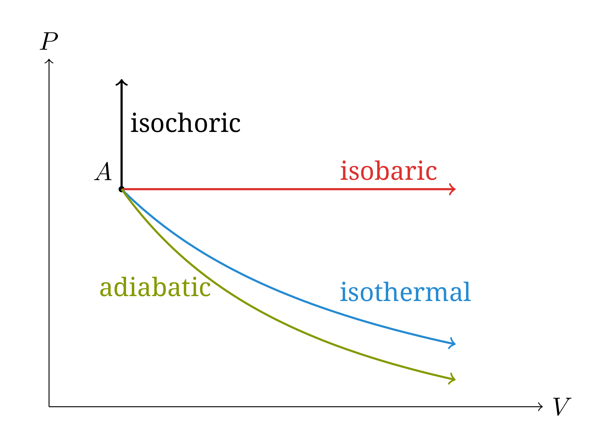
The four transformations encountered above take particularly simple forms in the $(P,V)$ plane.

An isochoric transformation, $V=V_0$, is represented by a vertical segment, while an isobaric transformation, $P=P_0$, is represented by a horizontal segment.

For an isothermal transformation, the equation of state gives $P(V)=nRT_0/V$: the curve is therefore a branch of a hyperbola.

Finally, an adiabatic transformation obeys the Laplace relation $PV^\gamma=\mathrm{const}$, that is, $P=K/V^\gamma$. Since $\gamma>1$, pressure decreases more rapidly with volume along an adiabat than along an isotherm. This can be seen directly by comparing, at the same point, the slopes

$$\left(\frac{dP}{dV}\right)_{\mathrm{isoth}} =-\frac{P}{V}, \qquad \left(\frac{dP}{dV}\right)_{\mathrm{ad}} =-\gamma\frac{P}{V}.$$

The adiabat is therefore “steeper” than the isotherm.

3.2. Two paths between the same states

The Clapeyron diagram now makes it possible to visualize a fundamental property established in the previous lesson: $U$ is a state function, whereas $Q$ and $W$ depend on the particular transformation.

Consider, for example, the two states

$$A=(P_0,V_0), \qquad B=\left(\frac{P_0}{2},2V_0\right).$$

The ideal gas equation gives $T_A=T_B=T_0$, with $T_0=P_0V_0/(nR)$. Since the internal energy of an ideal gas depends only on its temperature,

$$\boxed{\Delta U_{A\to B}=0}$$

for any transformation connecting $A$ to $B$. Let us now compare the two paths shown in Figure 2.

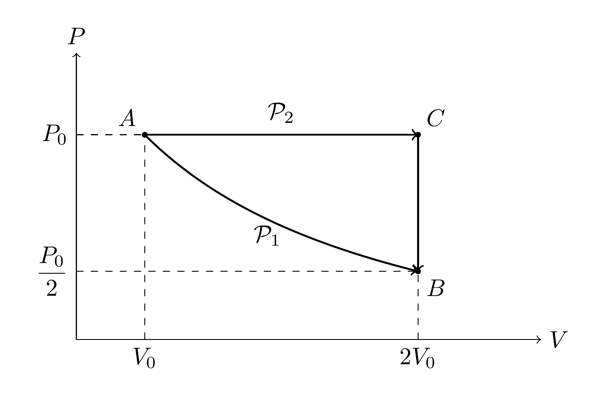
For the first path $\mathcal P_1$, which is a direct isothermal expansion, we have

$$W_1=-nRT_0\ln 2=-P_0V_0\ln 2.$$

Since $\Delta U=0$, it follows that $Q_1=-W_1=P_0V_0\ln 2$.

For the second path $\mathcal P_2$, the isobaric transformation $A\to C$ is performed first, followed by the isochoric transformation $C\to B$. The work received on the first branch is $W_{AC}=-P_0V_0$, while $W_{CB}=0$. Thus,

$$W_2=-P_0V_0, \qquad Q_2=P_0V_0.$$

We finally obtain

The two paths have the same endpoints and therefore the same change in internal energy, but they lead to different values of work and, by the first law, to different heat transfers.

3.3. Work as the area under the curve

The path dependence of work has an immediate geometric interpretation. For a quasi-static transformation represented in a Clapeyron diagram, the work received is

The integral $\int_A^B P\,dV$ represents the signed area under the curve describing the transformation. With our sign convention, the work received by the gas is the negative of this area.

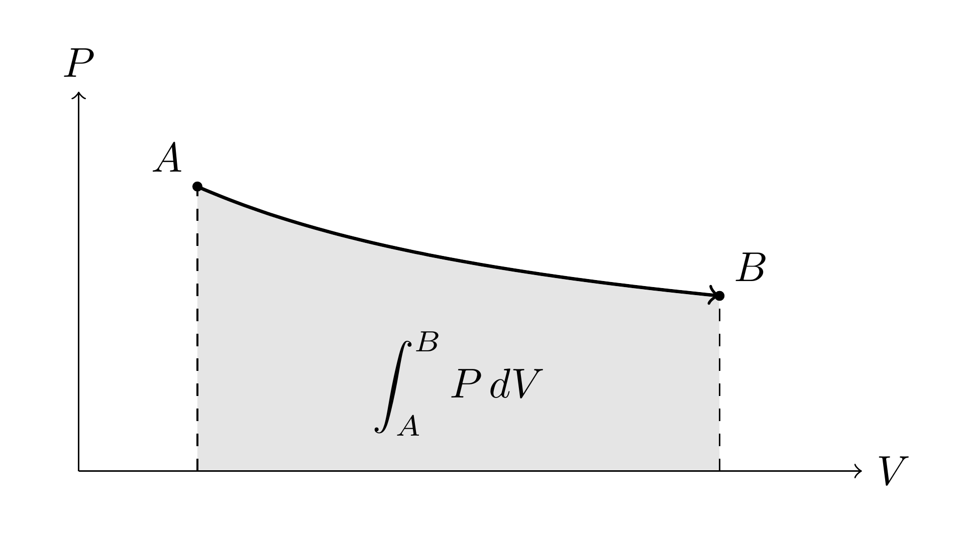
Here it is crucial to remember that the order of the limits determines the sign of the integral. During an expansion from $A$ to $B$, with $V_B>V_A$, we have

$$W[A\to B]=-\int_{V_A}^{V_B}P\,dV<0 :$$

the gas supplies work to its surroundings. During the reverse compression, the limits are interchanged and

$$W[B\to A] =-\int_{V_B}^{V_A}P\,dV =+\int_{V_A}^{V_B}P\,dV>0 :$$

the gas receives work. It is therefore essential to use an arrow to indicate the direction in which any curve plotted in a Clapeyron diagram is traversed.

This interpretation also provides a very simple explanation of why the two paths in Figure 2 lead to different values of work: the areas under the two curves are not the same.

3.4. Power cycles and refrigeration cycles

During a cyclic transformation, the system returns to its initial state. The cycle is therefore represented by a closed curve in the Clapeyron diagram.

Since $U$ is a state function, $\Delta U_{\mathrm{cycle}}=0$. The first law therefore requires $Q_{\mathrm{cycle}}=-W_{\mathrm{cycle}}$. Moreover,

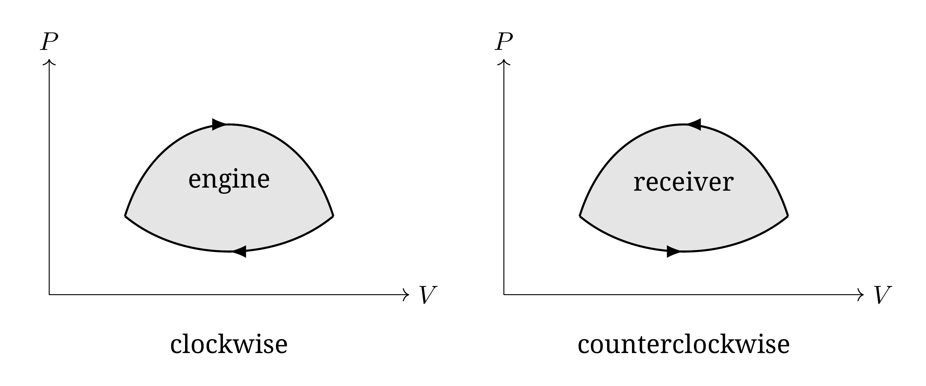
The preceding geometric interpretation then takes a particularly simple form: the absolute value of the work is equal to the area enclosed by the cycle. To see this, consider a cycle consisting of an upper branch $P_+(V)$ traversed from $V_1$ to $V_2$, with $V_1<V_2$, followed by a lower branch $P_-(V)$ traversed in the opposite direction, as in Figure 4. We have

$$\oint P\,dV = \int_{V_1}^{V_2}P_+(V)\,dV + \int_{V_2}^{V_1}P_-(V)\,dV = \int_{V_1}^{V_2} \bigl[P_+(V)-P_-(V)\bigr]\,dV.$$

This is the area under the upper branch minus the area under the lower branch, in other words the area enclosed by the cycle. For the clockwise path considered here, this integral is positive and the work received is therefore negative.

For a power cycle, the first law requires $Q_{\mathrm{cycle}}=-W_{\mathrm{cycle}}>0$: over the complete cycle, the gas receives a net amount of heat equal to the work it supplies to its surroundings.