Direction of Evolution, Equilibrium and Stability

The first law imposes the conservation of energy; the second law specifies the direction of possible evolutions through the increase of the total entropy. Let us now use this balance to study the spontaneous direction of heat or mechanical transfer, and then equilibrium and its stability. We will restrict ourselves to closed systems, each time distinguishing the system under study from the isolated composite system to which the second law applies.

1. The irreversibility of heat transfer

Consider two closed systems ${\mathcal{S}}_1$ and ${\mathcal{S}}_2$, of fixed volumes, brought into thermal contact. They need not be gases. The following argument is general. They exchange neither matter nor work, but can exchange heat. The composite system is assumed to be isolated. A weakly conducting wall makes the exchanges slow enough for each system to remain close to its internal equilibrium. Each one then evolves quasi-statically and has a temperature $T_i>0$ at every instant. We neglect the contributions of the wall to the energy and to the entropy.

At fixed volume and amount of matter, the fundamental relation gives, with $d{V}_i=0$,

Let $\delta Q_i$ denote the algebraic heat received by system $i$. Since no work is exchanged, $d{U}_i=\delta Q_i$, and since the composite system is isolated, the first law and the additivity of energy require $d{U}_1+d{U}_2=0$. Writing $\delta Q_{1\to 2}$ for the heat transferred from 1 to 2, counted as positive in that direction, we therefore have

By the additivity of entropy, the second law applied to the isolated composite system gives

When $T_1>T_2$, this inequality requires $\delta Q_{1\to 2}\ge 0$: the transfer therefore goes from hot to cold. If $T_1<T_2$, its direction is reversed, and the transfer again goes from hot to cold. We thus see how the second law imposes the direction of the possible exchanges, in agreement with everyday experience.

When $T_1\ne T_2$, any nonzero transfer in the allowed direction gives $d{S}_{\mathrm{tot}}>0$. The spontaneous transfer from hot to cold is therefore globally irreversible, even if each part evolves quasi-statically.

2. Entropy and equilibrium

Let us continue the previous example. Since the wall is conducting, the transfer continues as long as a temperature difference persists. Thermal equilibrium therefore requires $T_1=T_2$.

We then observe that $d{S}_{\mathrm{tot}}$ vanishes for any small redistribution of energy between the two bodies: the total entropy is stationary. This result motivates the general criterion that we will assume: at equilibrium, the entropy of an isolated composite system is stationary with respect to the small internal variations allowed by the constraints. In other words, its first-order variation vanishes. This criterion provides a necessary condition for equilibrium; it proves neither the uniqueness of the equilibrium nor the convergence of every evolution towards this state.

To illustrate it, consider a rigid, isolated cylinder containing two compartments of ideal gas separated by a movable, diathermal wall that is impermeable to matter. The wall moves without friction and is subject to no additional force. We neglect its own energy. Conservation of the total energy gives $d{U}_2=-d{U}_1$, while conservation of the total volume requires $d{V}_2=-d{V}_1$. The fundamental relation then gives

The wall allows both heat transfer and displacement: the redistributions of energy and of volume can therefore be varied independently to test stationarity. The aim here is to compare neighbouring states, not to describe the actual motion of the wall. At equilibrium, this variation must vanish for all such variations. Both coefficients vanish: we obtain $T_1=T_2$, and then $P_1/T_1=P_2/T_2$, that is,

These familiar conditions show the value of the stationarity criterion, but also the importance of the constraints. If the wall remains movable but becomes adiabatic, it forbids heat transfer while still allowing an exchange of work: $d{U}_1$ and $d{V}_1$ are then no longer independent variations. The two coefficients can therefore not be set to zero separately as before. Mechanical equilibrium still requires $P_1=P_2$, through the balance of forces on the wall, but this condition is not sufficient to impose $T_1=T_2$.

3. Equilibrium and stationarity of entropy

In the previous section, we assumed that the entropy of an isolated composite system is stationary at equilibrium: its first-order variation vanishes when the free parameters of the system are varied slightly while respecting the imposed constraints. Let us repeat this calculation for two subsystems that can also exchange particles. Each is assumed to be in internal equilibrium, and contributions from their interface are neglected. The composite system is isolated: its energy $U$, volume $V$ and particle number $N$ are fixed. The constraints therefore read

The parameters of each subsystem may nevertheless vary, provided their changes compensate one another:

The wall may impose additional constraints: if it is fixed, $d{V}_1=0$; if it is impermeable, $d{N}_1=0$. We must therefore specify the allowed exchanges to determine which parameters remain free.

Expressing the parameters of the second subsystem using the constraints makes the total entropy a function of $U_1$, $V_1$ and $N_1$:

The fundamental relation gives

If the three free parameters $U_1$, $V_1$ and $N_1$ can vary independently in both directions near equilibrium, stationarity requires the coefficient of each variation $d{U}_1$, $d{V}_1$ and $d{N}_1$ to vanish. We obtain in turn:

Equality of chemical potentials thus complements the thermal and mechanical equilibrium conditions already encountered. Each equality corresponds to an allowed variation. If the wall is impermeable, $d{N}_1=0$: stationarity then imposes no equality between ${\mu }_1$ and ${\mu }_2$.

For a permeable but fixed wall, note that at a common temperature, $T_1=T_2=T$, we simply have

which shows that if ${\mu }_2>{\mu }_1$, a transfer of particles from 2 to 1 ($d{N}_1>0$) increases entropy and therefore occurs spontaneously. As announced in the previous lesson, at a uniform temperature, matter tends to move from regions of higher chemical potential to regions of lower chemical potential, until the chemical potentials are equal at equilibrium.

4. Stability and concavity of entropy

Stationarity of entropy has given us the equilibrium conditions of an isolated system. Let us return to the two subsystems of the previous section: $U_1$, $V_1$ and $N_1$ are varied through the allowed exchanges, while the totals $U$, $V$ and $N$ are kept fixed. Stationarity of the total entropy around the equilibrium partition means that these variations do not change $S_{\mathrm{tot}}$ to first order.

Two descriptions must be distinguished here. On the equilibrium surface $S=S(U,V,N)$, in the four-dimensional space $(U,V,N,S)$, the fixed totals determine a single point: that of the equilibrium of the whole system. But these same totals allow many partitions between the two subsystems. To describe them, we need the additional parameters $U_1,V_1,N_1$, those of the second subsystem being imposed by the totals. The total entropy depends on this partition and is not necessarily equal to $S(U,V,N)$. The constrained maximum is taken over this set of partitions; it does not consist in varying the totals on the equilibrium surface.

Let us now examine what the second order tells us. If the entropy decreases strictly to second order in all nonzero allowed directions, the partition corresponds to a local maximum of the entropy. It is then locally stable: any small allowed deviation would decrease the entropy and therefore cannot occur spontaneously in the isolated system.

If, on the other hand, the entropy can increase in some directions and decrease in others around a partition where it is stationary, its graph has a saddle point. The system may have evolved spontaneously towards this equilibrium state, but it may also very easily move away from it spontaneously by further increasing its entropy: it is therefore an unstable state.

Second derivatives thus provide information on the local stability of equilibrium. But even a local maximum (locally stable) can be globally unstable, or, as we also say, metastable. Another partition of the energy, volume and particles between the subsystems may yield a higher total entropy, with the same totals and the same constraints. This is the analogue, in classical mechanics, of a system trapped around a local minimum of potential energy that is not a global minimum.

Stable thermodynamic equilibrium, by contrast, corresponds to the global maximum among all these partitions. The second order, which describes only the neighbourhood of the state under consideration, is not sufficient to establish this property, even though it helps characterize its local aspect.

4.1. The maximum entropy principle

The characterization of stable equilibrium that we have just presented is called the maximum entropy principle. It appears in Callen's Postulate II ^[1], Section 1.10.

This principle characterizes stable equilibrium; it does not assert that every spontaneous evolution reaches it, since a metastable state can persist. We will return to metastability in the study of phase transitions.

4.2. Concavity of S

How can this maximum over internal partitions impose a property on the equilibrium surface $S(U,V,N)$ itself? Take two portions of the same body, each in internal equilibrium, but not necessarily in equilibrium with each other. Let $X=(U,V,N)$ and $X_1=(U_1,V_1,N_1)$; the second portion then has the quantities $X_2=X-X_1$.

Each portion is described by the same fundamental function $S$: its quantities and its entropy define a point on the equilibrium surface of this body. Thus an internal partition of the whole system is described by two points on this surface, $(X_1,S(X_1))$ and $(X_2,S(X_2))$. If the system is additive, neglecting interface effects, their entropies add up:

The semicolon is a reminder that $X$ is fixed. The maximum principle then gives

The left-hand side describes the equilibrium of the whole system; the right-hand side describes its two portions before they reach mutual equilibrium.

Extensivity now allows us to go from this sum to a weighted average. Choose two reference states $X_A$ and $X_B$ on the same surface, then take a portion of size $\lambda$ of the first and a portion of size $1-\lambda$ of the second. Their quantities are $X_1=\lambda X_A$ and $X_2=(1-\lambda )X_B$, and their entropies are $\lambda S(X_A)$ and $(1-\lambda )S(X_B)$. It is this construction that brings out concavity.

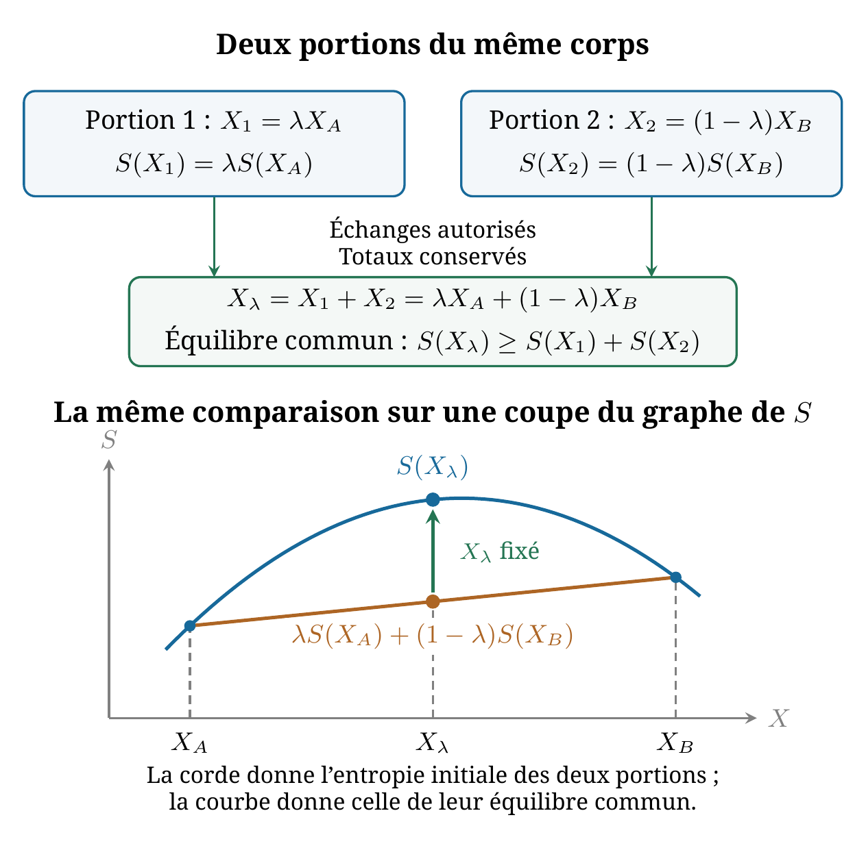
On this graph, the point on the chord and the point on the curve at $X_{\lambda }$ correspond to the same totals. The first represents the entropy of the two separate portions, the second that of their common equilibrium. Since the reference states and the proportion $\lambda$ are arbitrary, this comparison at fixed totals constrains the shape of the entire equilibrium surface.

We thus return to second derivatives, but their role has become clearer. At the beginning of the section, those of $S_{\mathrm{tot}}$ with respect to the internal parameters provided information on the local stability of a partition, at fixed totals. Thanks to additivity and extensivity, this requirement also translates into a condition on the second derivatives of the fundamental function $S(U,V,N)$. Imposed at every point and in every direction of a convex domain, this condition characterizes the concavity of $S$ over the whole domain. A local condition at a single point would not be sufficient.

Concavity is easy to visualize for functions of a single variable. For such a sufficiently smooth function, concavity is equivalent to a second derivative that is negative or zero at every point. In higher dimensions – here $S$ is a function of three variables – the geometric interpretation remains the same: the graph of the function lies above every chord joining two of its points. If the function is sufficiently differentiable, this means that its second derivative is negative or zero in every direction. Checking this condition separately for each variable, with the others held fixed, is therefore not sufficient: one must also consider the directions in which several variables vary together. The correct analytical criterion is in fact the following:

In practice, we will only need functions of two or three variables in the rest of this course. We assume here that, in this case, the preceding criterion translates into the following conditions, to be checked at every point.

We will apply these criteria to entropy in Lesson 9, once the calorimetric and thermoelastic coefficients have been introduced.

4.3. The energy minimum

Since the temperature is positive, the equation of state $1/T={\left(\frac{\partial S}{\partial U}\right)}_{V,N}$ of Lesson 7 implies

$S$ is therefore strictly increasing in $U$ at fixed $V$ and $N$: we can invert $S(U,V,N)$ to obtain $U(S,V,N)$. The concavity of $S$ then translates, conversely, into a convexity of the energy $U(S,V,N)$ (on any convex domain on which it is defined).

5. Summary: the geometry of thermodynamics

Concavity therefore constrains the shape of the fundamental equation. Let us now look at the surface it defines. A function $S=S(U,V,N)$ assigns an entropy to each admissible triple $(U,V,N)$. Its graph is a three-dimensional object embedded in the four-dimensional space $(U,V,N,S)$. It is therefore impossible to represent it entirely on a sheet of paper. If $N$ is fixed, what remains is a two-dimensional surface $S=S(U,V)$ that can be represented in a three-dimensional space. Extensivity moreover gives this graph a cone structure: together with each point $(U,V,N,S)$, it contains the ray $(\lambda U,\lambda V,\lambda N,\lambda S)$, for $\lambda >0$. The surface described by $s=s(u,v)$ fixes the shape of this cone; $N$ sets its scale.

This surface gathers the equilibrium states. What, then, does a transformation represent? A real, rapid transformation generally passes through states that are not equilibrium states. The temperature or the pressure may not be uniform, and a single point on the surface is no longer enough to describe the system. Equilibrium thermodynamics represents only the initial state and the final state.

A quasi-static transformation is an idealization in which the system remains, at every instant, arbitrarily close to an equilibrium state. In the ideal limit, it is represented by a curve drawn on the equilibrium surface. This is not, however, enough to make it reversible. A piston can move arbitrarily slowly while being subject to friction. The system then passes through a succession of well-defined states, but entropy is produced and it is impossible to restore the system, the surroundings and the devices without any other effect.

In the sense of Lesson 6, a locally reversible transformation passes through a succession of equilibrium states, each step of which, including the exchanges with the surroundings, can be reversed by an infinitesimal change in the constraints. It is quasi-static, produces no entropy and is also globally reversible. Global reversibility, for its part, is defined by the possibility of restoring the system and all of its surroundings, without requiring the initial path to be retraced.

The distinction between quasi-staticity and local reversibility can therefore not be read off by placing a curve slightly above or exactly on the equilibrium surface. In both cases, the idealized thermodynamic curve is drawn on this surface. Entropy production and the possibility of reversing each step, including its external effects, are additional information.

We now have two equivalent descriptions, $U(S,V,N)$ and $S(U,V,N)$, together with the relations linking their derivatives. But the natural variables of these two functions are not always those that experiment holds constant. A thermal reservoir imposes $T$, not $S$. An atmosphere or a loaded piston imposes $P$, not $V$. It thus remains to understand how to change variables without losing the information contained in the fundamental relation. Lesson 9 will first relate its derivatives to measurable coefficients; its appendix gathers the rules of differential calculus that are useful from that lesson onwards. Lesson 10 will then construct the potentials suited to the experimental constraints.

6. Summary: the assumptions of the theory

With the fundamental relation, the structure of equilibrium thermodynamics is in place. The assumptions on which it rests were laid down over the course of the lessons, often at the precise moment they were needed. Here they are, gathered together.

This inventory allows us to clarify the remark “A law is not an axiom” in Lesson 2. Taken in isolation and in their usual form, the two laws are not axioms: they say neither what a state is, nor what structure the state space has, nor how systems combine. Supplemented by the seven other assumptions, however, they do play that role. This is how we treated them in Lessons 4 and 6: from the Clausius statement, we derived theorems (Carnot's theorems, the Clausius inequality, the increase of the entropy of an isolated system), not new laws.

The status of axiom moreover depends on the chosen starting point. Callen directly postulates the existence of entropy, its additivity, its increase with energy and the maximum entropy principle ^[1]. His postulates thus cover assumptions 1, 7, 8 and 9, the eighth in a stronger form. The Clausius statement then becomes a theorem: the spontaneous transfer of heat from hot to cold follows from the maximum entropy principle. Finally, our list is not an axiomatic system in the strict mathematical sense. Notions such as the “sole effect” in the Clausius statement, thermal reservoirs or locally reversible paths remain intuitive in it. The axiomatic formulations mentioned in Lesson 2 aim precisely to define them; we will return to them in the second part of the book.

7. Going further

7.1. Absolute zero and the third law

In the ordinary systems considered so far, the temperature is positive. The function $U(S,V,N)$ is then increasing in $S$, which allows us to pass from the energy representation to the entropy representation. This does not mean that absolute zero results from a mere choice of sign. The absolute temperature scale was constructed from the second law, and $T=0$ is a limit of it.

The third law specifies the behaviour of entropy as this limit is approached. In Nernst's formulation, the entropy changes associated with an isothermal transformation tend to zero as $T$ tends to zero. The entropy therefore tends to a constant independent of the continuous macroscopic parameters. In Planck's formulation, valid for a perfect crystal with a unique ground state, this constant is chosen equal to zero:

If the ground state is degenerate or if some disorder remains frozen in, a residual entropy may persist. The claim that the entropy of every system necessarily tends to zero would therefore be too strong.

Another formulation associated with the third law is the unattainability of absolute zero: no finite sequence of physical transformations makes it possible to reach exactly $T=0$. A system can be cooled ever closer to this temperature, but the point $T=0$ remains a limit.

The Sackur-Tetrode formula seems to contradict this result. Using $U=3N{k}_{B}T/2$, it indeed gives

as $T$ tends to zero, and hence $S\to -\infty$. The contradiction is only apparent. The Sackur-Tetrode formula describes the dilute classical regime. When the temperature becomes low enough, the quantum states occupied by the particles overlap and the classical approximation ceases to be valid. One must then use Bose-Einstein or Fermi-Dirac statistics.

8. References