The First Law of Thermodynamics

The previous lesson introduced thermodynamic systems, equilibrium states and state functions. We now turn to a central question: how can the energy of a system be incorporated into this macroscopic description?

Some courses treat this question too quickly: the first law is presented as a mere statement of energy conservation, and the energy balance formula follows immediately, with no further justification. We shall meet these formulas in Sections 3 and 4.3, and the reader in a hurry may indeed turn to them directly (see also the short summary in Section 7).

The construction leading to these formulas is, however, a subtle one. First, the first law asserts more than energy conservation, which (nowadays) seems obvious from a microscopic point of view. We shall show that this law in fact bridges the logical gap between the existence of an energy $U_{\mathrm{micro}}$ defined mechanically on a space of some $6N$ coordinates, and that of a state function $U_{\mathrm{th}}$ depending on only a handful of macroscopic variables.

We shall then show that the additivity of energy is a further assumption, needed to pass from the conservation of energy of an isolated system to an energy balance at the boundary of a closed system. It is this last step that finally makes the epistemic and logical status of heat precise: heat is defined as whatever transfer of energy remains in that balance once the macroscopic work done on a closed system has been accounted for, $Q \equiv \Delta U - W$.

In this lesson we first consider closed systems: no matter crosses their boundary. The reason is simple: in an open system, matter itself carries energy across the boundary and complicates the energy balance. Open systems will be treated later in the course.

1. The microscopic internal energy

Consider a classical, non-quantum and non-relativistic system in an inertial frame¹. Consider $N$ point particles of masses $m_i$, positions $\vec r_i$ and velocities $\vec v_i$. At any instant, its microscopic state is completely determined by

where $\Gamma$ denotes the classical phase space of the system, of dimension $\dim\Gamma=6N$ in this simple model. We assume that all internal forces, for instance the attractive or repulsive forces between molecules, are conservative. A total potential energy may then be associated with them, $E_p^{\mathrm{int}}(\vec r_1,...,\vec r_N), \, \mathrm{with} \,\,\, \vec F_i^{\,\mathrm{int}} =-\nabla_{\vec r_i}E_p^{\mathrm{int}}$. The system may also be subject to external conservative forces, its weight for instance. In the same way, an external potential energy $E_p^{\mathrm{ext}}(\vec r_1,...,\vec r_N)$ is associated with them.

The system need not be at rest in the chosen frame. At every instant one may define its center of mass and its velocity $\vec V$, which may itself depend on time. Introducing the total mass of the system and the velocities relative to the center of mass,

the total kinetic energy may then be written as

Expanding the square, one finds that the cross terms cancel exactly, since $\sum_i m_i\vec u_i=\vec 0$. This result is known as König's theorem in classical mechanics:

Hence:

The total kinetic energy therefore always splits² into the macroscopic kinetic energy of the center of mass, and that of the residual relative motions, the “disordered” ones, which make up what is called thermal agitation.

Collecting the various terms, the total mechanical energy finally reads

Remark: the term $E_{\mathrm{int}}^{\mathrm{autres}}$ collects the contributions of the internal degrees of freedom that this minimal point-particle model does not describe, for instance the rotational or vibrational degrees of freedom of the molecules. If these are modeled explicitly, the phase space $\Gamma$ must be enlarged accordingly.

In what follows we shall consider systems that are macroscopically at rest, free of global rotation, and whose external potential energy does not change. Up to a choice of origin, we may therefore write

We now introduce the thermodynamic energy state function, provisionally written $U_{\mathrm{th}}$, and explain why it must not be identified a priori with $U_{\mathrm{micro}}$.

2. The thermodynamic internal energy

Take as our system a saucepan of water placed on a hotplate. We remain within the simple framework described above: the saucepan is macroscopically at rest and its external potential energy does not change. We may therefore write $E_{\mathrm{tot}}=U_{\mathrm{micro}}$ up to a constant.

When the water is heated, no macroscopic kinetic energy appears and the saucepan does not move. Granting the strict conservation of energy in all its forms, the energy supplied to it must therefore end up in its microscopic internal energy:

Thermodynamics seeks to describe exactly the same change. We should therefore like to construct a quantity $U_{\mathrm{th}}$ such that

The solution looks obvious. Is it not enough to identify the thermodynamic internal energy with the microscopic internal energy?

Such an identification would in fact be mathematically incorrect, since the two functions do not have the same domain of definition. $U_{\mathrm{micro}}$ is a function defined on phase space and depends on at least $6N$ variables, whereas $U_{\mathrm{th}}$ depends only on a small number $d$ of independent variables describing the equilibrium state $X=(x^1,...,x^d)\in\mathcal E$ (recall that the $x^i$ are macroscopic state variables, such as temperature, pressure or volume).

The two functions must nevertheless be related in such a way that $U_{\mathrm{th}}(X)$ represents, at the macroscopic scale, the internal energy corresponding to the equilibrium state $X$. How this dimensional reduction works must be explained. The question is a deep one and goes beyond the scope of this introductory course. A microscopic description is needed if one wishes to derive this passage between the two scales. Subsection 6.2, which lies outside the syllabus, outlines how statistical physics solves the problem.

From a strictly thermodynamic point of view, however, no justification of this microscopic identification is possible, and the existence of $U_{\mathrm{th}}$ as a function of a few macroscopic variables only must be postulated. This will be the role of the first law of thermodynamics, which therefore asserts not only the conservation of energy, but also, and above all, that this energy can be represented at equilibrium by a state function defined on the macroscopic space $\mathcal E$.

Once the $d$ independent state variables $x^i$ have been chosen, say ($T$, $V$, $N$) for an ideal gas, the function $U(T,V,N)$ defines a scalar field on the state space; in the enlarged space of coordinates $U,T,V,N$, its graph is a hypersurface, called the equilibrium surface, whose role in the rest of this course will be crucial, cf. Figure 1.

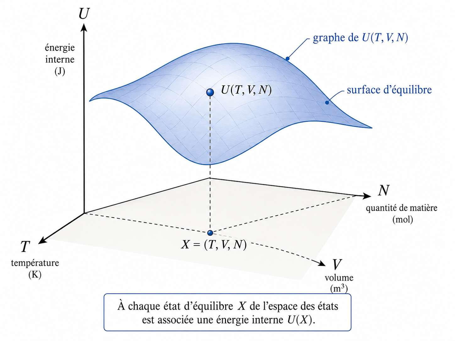
Let us finally note an immediate corollary, which illustrates the difference between $U_{\mathrm{th}}$ and $U_{\mathrm{micro}}$ rather well: in the equilibrium thermodynamics developed here, the thermodynamic internal energy is in general not defined outside equilibrium states. During a violent process undergone by a gas, for instance, it is possible, and indeed common, that no single temperature or pressure can be assigned to it any longer. In that case the thermodynamic internal energy $U_{\mathrm{th}}$ cannot be assigned to it directly either, since it is defined only on the space of equilibrium states $\mathcal E$. The difficulty is not that the energy has ceased to exist, for its microscopic energy remains perfectly well defined at every instant, but simply that the system is no longer represented by a point $X\in\mathcal E$.

All this being said, from the next section onwards the mechanical function $U_{\mathrm{micro}}$ will no longer appear directly: we shall simply write $U$ for the thermodynamic internal energy $U_{\mathrm{th}}$, understood to be defined on the space of equilibrium states only.

3. The first law of thermodynamics

The previous section has done much of the groundwork; we can now state:

The regularity of the function $U$ is likewise a non-trivial assumption. In practice, $U$ may be taken to be $\mathcal C^\infty$. Since $U$ is determined only up to a constant, because of the potential energies involved in equality 3, only its variations carry physical meaning. For simplicity, we shall restrict ourselves in what follows to processes in which the macroscopic kinetic and potential energies do not change. We then have $\Delta E_{\mathrm{tot}}=\Delta U$.

Consider now a closed system $S$, which may exchange energy, but not matter, with its surroundings. The global system

can always be embedded in an isolated system. The first law then imposes

Under the further assumption that energy is additive, that is, that their interaction energy is negligible, we have $E_{S'}=E_S+E_{\mathrm{Ext}}$, so that

The assumption of additivity thus turns the conservation of energy into a balance between subsystems: whatever energy is gained by the system is lost by its surroundings, and conversely. It remains to specify how this energy can be transferred across the boundary of the system. We shall distinguish two modes of transfer: work, written $W$, which has an independent definition inherited from mechanics, and heat, written $Q$.

The energy balance will then take the form

where $W$ denotes the work received by the system and $Q$ the heat received by it.

Note that the assumption that energy is additive is not a trivial one. At an elementary level, it may simply be granted for the usual thermodynamic systems. It is not always valid, however. Long-range interactions in particular can defeat both the additivity and the extensivity of energy at once, see Section 6.4.

It now remains to define these two modes of transfer. Before that, it is essential to note a sign convention, an entirely standard one, that will be used throughout this course.

4. Work, heat and the energy balance

4.1. Work

One of the advantages of work is that it has a definition independent of thermodynamics, inherited from mechanics. When an external force $\vec F_{\mathrm{ext}}$ acts on a point of the boundary of the system and that point is displaced by $d\vec r$, the elementary work supplied by this force, and therefore received by the system, is

For an extended system, the contributions of all the external forces doing work on its boundary must be summed.

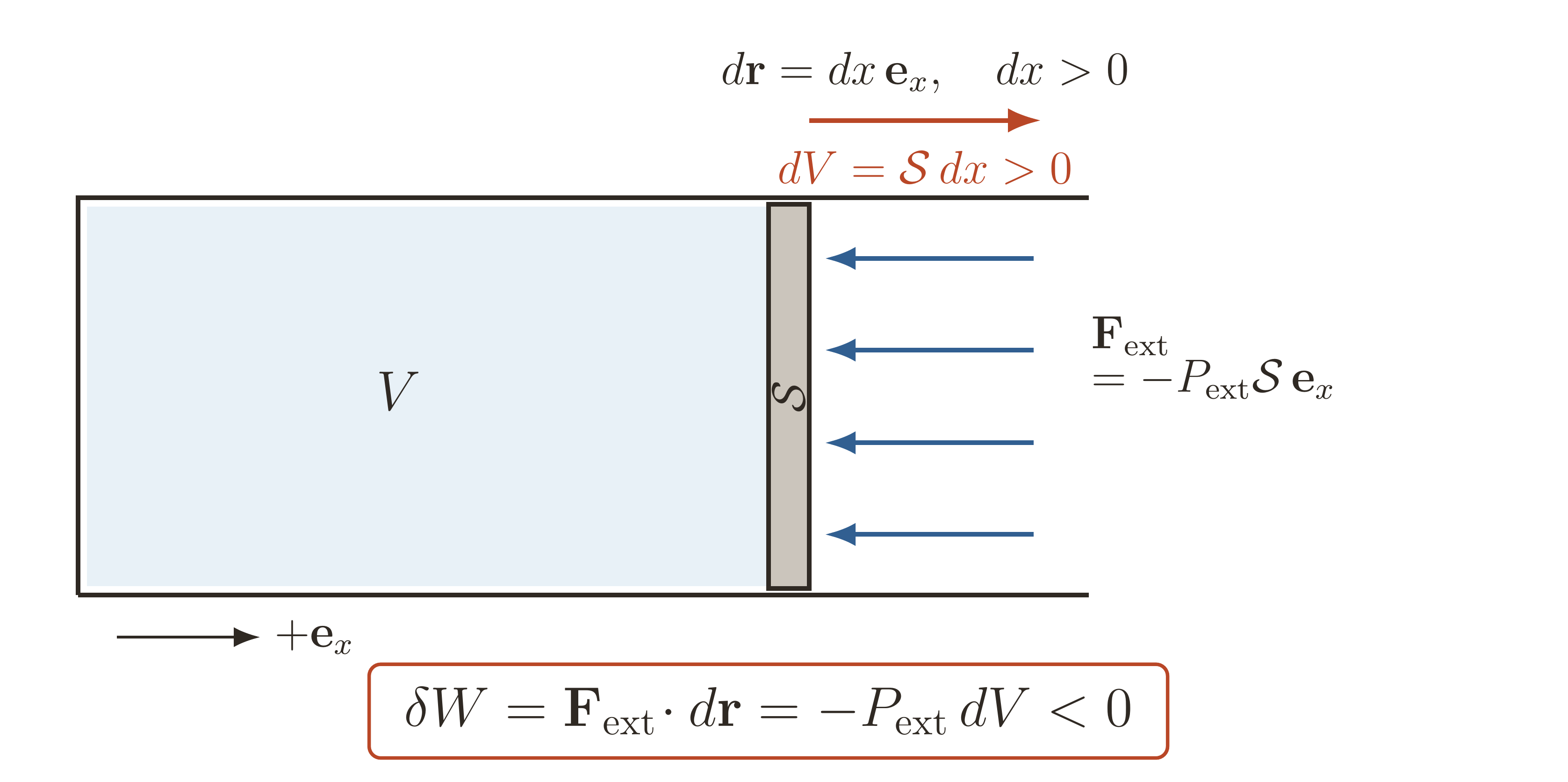
The case that will serve us most often in practice is that of a fluid contained in a vessel with one movable wall, which leads us to evaluate the work of the pressure forces. Consider a gas enclosed in a cylinder by a flat piston of cross-section $\mathcal S$, cf. Figure 2. The $x$ axis points outward from the gas. When the piston is displaced by an amount $dx$, the volume changes by

Let $P_{\mathrm{ext}}$ denote the external pressure exerted on the boundary of the gas. The force received by the gas is directed inward and is

The elementary work received by the gas is therefore

that is

The banker's rule makes the sign immediate to check. In a compression, $dV<0$, hence $\delta W>0$: the gas receives work. In an expansion, $dV>0$, hence $\delta W<0$: the gas supplies work to its surroundings.

Note that the pressure appearing in this formula is indeed the pressure external to the system, which in general has no reason to equal the pressure of the gas itself. This is particularly important to keep in mind for violent, out-of-equilibrium processes, where the internal pressure is in general not even defined.

Integrating, we obtain the following formula for a finite process $A \to B$ during which the external pressure is known:

This integral shows that, in order to compute the total work, the value of $P_{\mathrm{ext}}$ must be known all along the process. This has a major consequence: the work can in general not be determined from the initial and final states $A$ and $B$ alone: its expression depends on the process followed.

Three particular cases are worth pointing out here.

1. If $P_{\mathrm{ext}}$ is constant, then $W_{\mathrm{pression}}[A\to B] = -P_{\mathrm{ext}}\Delta V$.
2. Along an isochoric process, $dV=0$, and the work of the pressure forces vanishes: $\delta W_{\mathrm{pression}}=0$ and $W_{\mathrm{pression}}[A\to B]=0$.
3. In an expansion into a vacuum, $P_{\mathrm{ext}}=0$, so the work of the pressure forces vanishes as well.

4.2. Heat

Work cannot be the only mode of energy transfer, since heating a gas held in a rigid vessel raises its temperature and its energy without any external work being done. Energy has therefore crossed the boundary of the system without having been transferred as work. This second mode of energy transfer is called heat, or heat transfer.

In the construction adopted here (see Subsection 6.1 for an equivalent alternative construction), for a physical process $A \to B$ connecting two equilibrium states $A$ and $B$, once all the work terms received by the system have been identified, the heat received is defined by

so that we recover the relation announced above,

Since the work depends on the path of the process $A \to B$, while the energy change $\Delta U = U(B)-U(A)$ does not, the amount of heat exchanged must necessarily depend on it as well.

In thermodynamic language, one says that the internal energy $U$ is a state function (by postulate), whereas the work $W$ and the heat $Q$ are not. Recall what this means: the fact that $W$ and $Q$ cannot be functions of the state of the system at a given instant means that the system does not possess “an amount of work or of heat”; rather, $W$ and $Q$ are transfers of energy at its boundary during some process $A \to B$, exactly what we were after, in view of the various experiments described in Lesson 2.

Let us note that in a cyclic process $A \to A$ the system returns to its initial state, so that

The first law then imposes

A cyclic machine can therefore not supply work indefinitely without receiving an equal amount of energy from its surroundings. This is, historically, what is called the impossibility of perpetual motion of the first kind.

4.3. Differential form of the first law

The relation

connects two equilibrium states $A$ and $B$. It always holds, in the sense that it does not require the intermediate states themselves to be representable by points of the space of equilibrium states $\mathcal E$. If the process is a violent one, the system may temporarily leave the equilibrium surface defined over $\mathcal E$, while $U(A)$ and $U(B)$ remain perfectly well defined.

One special case must now be spelled out. Suppose the process is quasi-static. At every instant the system is then, by definition, in an equilibrium state. Such a process can be represented by a path

made of infinitesimally close equilibrium states, which never leaves the equilibrium surface. Since $U$ is a state function that is differentiable on $\mathcal E$, its change between two infinitesimally close states is an exact differential, written $dU$.

We then write $\delta Q$ and $\delta W$ for the corresponding elementary transfers of heat and work. In this case the first law takes the form

The difference in notation between $d U$ on the one hand and $\delta W$ or $\delta Q$ on the other is not merely cosmetic. It indicates that the former is an exact differential while the latter two are not, which is the mathematical counterpart of the fact that the energy change does not depend on the path followed, whereas $Q$ and $W$ do. The next section reviews, for the newcomer, the mathematics needed to grasp this crucial point.

In the particular case where the only work is that of the pressure forces, and where $P_{\mathrm{ext}}$ may be identified with the pressure $P$ of the system, this relation becomes

5. Exact and inexact differential forms

This section gathers the minimum of mathematics needed to give a precise meaning to the distinction between $dU$ on the one hand, and $\delta Q$ and $\delta W$ on the other. Readers already familiar with it may skip it.

5.1. The differential of a function

Let $f$ be a function of the variables $x^1,...,x^d$, assumed differentiable. Its differential is the expression

which measures the change of $f$ when one moves from the point $X$ to the neighboring point $X+dX$. The essential point is the following: if one follows a path $\gamma$ from a point $A$ to a point $B$, then summing all these elementary changes gives

In particular, along a closed path we have:

5.2. Differential forms

Consider now an expression of the same kind, which must on no account be confused with the differential of a function. Let $A_i(x^1,...,x^d)$ be arbitrary functions. We define $\omega$ by

Such an object is called a differential form. Once the functions $A_i$ are given, integrating it along a path $\gamma$ raises no difficulty. But nothing guarantees that there exists a function $f$ of which $\omega$ is the differential, that is, such that $A_i=\partial f/\partial x^i$ for every $i$.

• If such a function $f$ exists, the form is said to be exact, and one writes $\omega = d f$. The integral $\int_\gamma\omega = \int_\gamma df = f(B)-f(A)$ then depends only on the endpoints.
• Otherwise the form is said to be inexact, and it is then written $\delta\omega$ rather than $\omega$, as a reminder that it is the differential of no function. (Mathematicians would simply write the form as $\omega$.)

5.3. Schwarz's criterion

A simple test for deciding whether a differential form is exact is Schwarz's criterion. For simplicity we work with two variables (the generalization is immediate), with

If $\omega$ were exact, we would have $A=\partial f/\partial x$ and $B=\partial f/\partial y$, hence

since the order of differentiation is immaterial for a twice continuously differentiable function. We thus have a convenient test:

Up to subtleties that will not arise in thermodynamics, the converse holds as well.

5.4. Example: the work of the pressure forces

When the elementary transfers can be expressed in terms of the state variables along the quasi-static path, $\delta Q$ and $\delta W$ become differential forms on $\mathcal E$, and one can check whether they are exact or not.

By way of example, take $n$ moles of an ideal gas undergoing a quasi-static process, with $P_{\mathrm{ext}} = P$. We then have $\delta W=-P\,dV$. Since $P=nRT/V$, the elementary work reads

identifying $x=T$ and $y=V$. This is indeed a differential form defined on the state space. Schwarz's criterion gives

The two cross derivatives are not equal: the elementary work is indeed not an exact differential. There is therefore, in this case, no state function $W(T,V)$ of which $\delta W$ would be the change, and the work received between two states does depend on the path followed. The same reasoning applies to $\delta Q=dU-\delta W$: since $dU$ is exact and $\delta W$ is not, their difference cannot be exact either.

6. Going further

This section gathers the more advanced considerations announced earlier. It may be skipped on a first reading.

6.1. Two possible constructions of the first law

We have chosen here the following logical order: the existence of the state function $U$ is postulated by the first law, work is defined independently by mechanics, and heat is then defined by the balance

A remarkable fact follows. If the process is adiabatic, then $\Delta U = W$, which forces the adiabatic work $W_{\mathrm{ad}}$ to be, in its turn, always independent of the path followed.

This points to another possible construction of the internal energy: an operational one, hence independent of any microscopic consideration, and as it happens closer to the historical route. One begins by characterizing adiabatic processes without introducing the quantity $Q$ beforehand, so as to avoid any circularity in the reasoning.

The idea is a clever one: what is defined is not the transfer itself, but the apparatus. A wall is said to be adiabatic when the state of the system it encloses can be changed only by moving the external mechanical coordinates, that is, the piston, a stirrer or an electric current. The test is then direct: one holds these coordinates fixed and alters the surroundings arbitrarily, by plunging the enclosure into an ice bath, say, or bringing it close to a flame. If no state variable of the system changes, then the wall is adiabatic.

This characterization involves only states and mechanical displacements, never a transfer of energy: it therefore precedes any notion of heat. In practice, one approaches it by good insulation, or by working fast compared with the thermal relaxation time.

The work received, for its part, is measured in a purely mechanical or electrical way. This is the whole empirical content of Joule's experiments, carried out between 1843 and 1850 and repeated since with ever greater precision: a mass $m$ falling through a height $h$ supplies $mgh$, with no heat transfer involved. All the arrangements he devised and built in an adiabatic enclosure in the above sense (paddle wheel, heating resistor or compression of a gas) led him to the same conclusion: the same work supplied produces the same change of state, which for him constituted “the mechanical equivalent of heat”, as explained in Lesson 2. Joule was thus the first to show (an experimental indication of the fact) that adiabatic work does not depend on the path followed.

It was then Carathéodory, in 1909 ^[2], and above all Born, in 1921, who proposed to elevate this experimental fact into a postulate. Granting it, it becomes easy to construct a state function $U$ by setting

and then to define heat by difference for general processes, as we have done.

This construction is adopted in many textbooks, notably those of Pippard ^[3] and Callen ^[4]. It is equivalent to ours: postulating $U$ and then deducing the path-independence of adiabatic work is equivalent to postulating the path-independence of that work and then constructing $U$. A detailed account of this conceptual evolution, from Joule to Carathéodory and Born, will be found in Rosenberg ^[5].

6.2. Micro- and macrostates

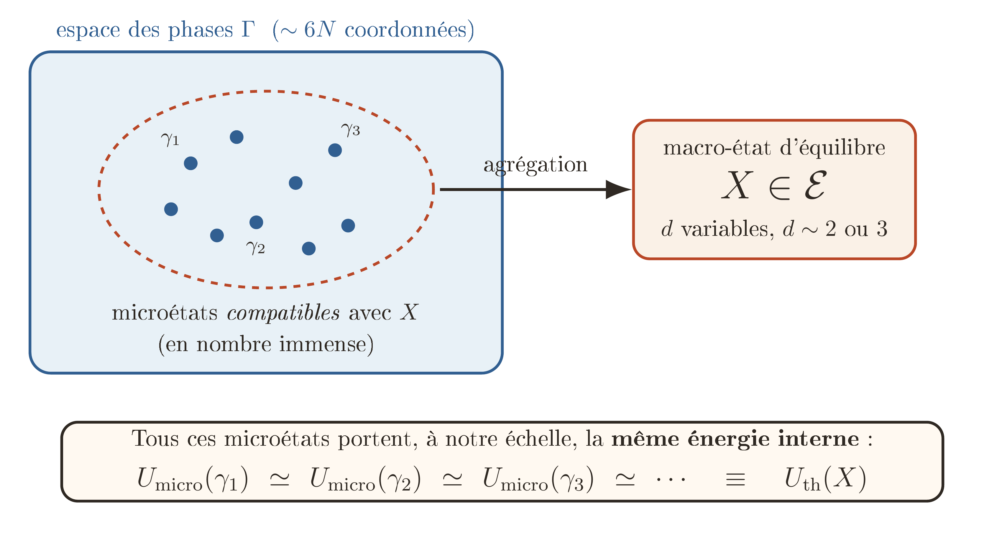
If one does not follow the operational route described above, then Section 2 has brought a fundamental question to light: how can an energy defined on a space of $6N$ coordinates be reduced to a function of only a few macroscopic variables? Statistical physics constructs this passage between the two scales. Its outline is as follows.

In statistical physics, a point $X$ of the space of equilibrium states $\mathcal E$ is called a macrostate. To one and the same macrostate there generally corresponds a gigantic number of microstates $\gamma\in\Gamma$ compatible with the same macroscopic constraints.

One then shows that the energies of these microstates are distributed extremely narrowly about their mean value as $N\to\infty$, the so-called thermodynamic limit. In other words, the relative fluctuations of the energy tend to zero:

One may then set $U_{\mathrm{th}}(X)= \langle U_{\mathrm{micro}} \rangle_X$, the average being taken over all microstates compatible with the macrostate. It is the concentration just mentioned that gives this definition its meaning. At every instant the system occupies a single microstate, not the average: only because nearly all of them carry the same energy can one speak of the energy of the macrostate, and can two identical preparations yield the same measurement.

One may picture the situation by imagining that to a macrostate there corresponds a very large collection of microstates that are microscopically different but macroscopically indistinguishable. This picture resembles that of an equivalence class on phase space. The precise construction will, however, be slightly different, and will involve a probability distribution on phase space.

The following figure summarizes this procedure.

6.3. Generalized work terms

The various forms of work met above share a common structure. We have seen the forms

for pressure work,

for the stretching of a wire, and again

for surface work. Note that in every case the quantity being differentiated is extensive, while its prefactor is intensive. Generalizing, we shall write any mechanical work term in the form

where $\nu_i^{\mathrm{ext}}$ denotes the external generalized force (generally intensive) conjugate to the coordinate $x^i$ (generally extensive), with the sign matching our convention.

When the external generalized forces can be identified with the corresponding thermodynamic forces of the system (for example $P_{\mathrm{ext}}=P$), the first law may then be written in the form

6.4. Extensivity of the internal energy

In the previous lesson we presented the internal energy as an extensive quantity: multiplying the size of a homogeneous system by a factor $\lambda$, at fixed intensive variables, multiplies its energy by $\lambda$,

This property is not postulated by the first law. It is a further assumption, which we shall often make, but which does not always hold. One indeed expects the presence of long-range forces between the constituents of the system, gravitational ones in particular, to ruin its extensivity.

Let us make this precise. Consider $N$ constituents distributed at constant density in a space of dimension $D$, and suppose that their interaction potential energy behaves as

At fixed density $\rho=N/V$, the typical linear size of the system grows as

Let us now evaluate the total interaction energy in three steps.

Counting the neighbors.

Fix one constituent and ask how many others lie at a distance between $r$ and $r+dr$. This is the density times the volume of the corresponding shell:

where $S_D$ denotes the area of the unit sphere in dimension $D$, that is $4\pi$ in three dimensions.

Summing over distances.

Each of these neighbors contributes $E_p(r)\sim r^{-\alpha}$. The interaction energy of a single constituent with all the others is therefore

The lower bound $a$ is the minimum distance of approach, below which the $1/r^\alpha$ law ceases to hold and which prevents the integral from diverging as $r\to0$. The upper bound $L$ is the size of the system: there is no neighbor beyond it.

Summing over constituents.

We multiply by the number of constituents (dividing by two so as not to count each pair twice):

where the geometrical factor $S_D/2$ has been absorbed into the order of magnitude. Let us now look at the value of the integral:

If $\alpha>D$, the exponent is negative: the integral converges as $L\to\infty$ and is dominated by its lower bound, hence of the order of the constant $a^{D-\alpha}/(\alpha-D)$. If $\alpha<D$, it is on the contrary dominated by its upper bound and is of the order of $L^{D-\alpha}=N^{1-\alpha/D}$. Finally, in the case $\alpha=D$, the antiderivative is a logarithm and the integral equals $\ln(L/a)=\tfrac1D\ln N$. Substituting, we thus obtain

Physically, the interpretation is clear. When $\alpha>D$, the forces are short-ranged: the decay of $E_p$ outweighs the growth in the number of neighbors. Each constituent feels only its immediate neighborhood, so that its energy does not depend on the size of the system, and the total is proportional to $N$, which is extensive.

When $\alpha\leq D$, the opposite happens: the distant neighbors, far more numerous, win out, each constituent feels the system as a whole, and its own energy grows with the size of that system. The total then grows faster than $N$, and extensivity is lost. Sufficiently short-ranged interactions therefore lead naturally to an extensive energy, whereas long-range interactions can destroy that property.

In three-dimensional Newtonian gravity, for instance,

and the above estimate gives, at fixed density,

The minus sign, which the order-of-magnitude argument does not by itself provide, reflects the attractive character of gravity.

The extensivity of energy will be used extensively in the rest of this book. Gravity is of course universal, but it is a very weak force: when studying two volumes of gas brought into contact, it can be neglected in practice. On the other hand, the internal forces within the gas, of van der Waals type, decay very fast (as $1/r^6$), so that extensivity is in that case very nearly exact.

For the description of so-called self-gravitating systems (stars, galaxies, ...), on the other hand, gravity is of course the essential ingredient, and the whole thermodynamic analysis must be taken up again from the start, since the extensivity of energy is necessarily lost. As a result, the thermodynamics of such systems is almost a subject of its own, and displays unexpected behavior: a star that radiates energy away, for instance, heats up instead of cooling down. We shall return to this in the advanced part of the book.

7. Summary

Let us summarize what this lesson has set up, and what will be used throughout what follows.

• The first law postulates the existence of a state function $U:\mathcal E\longrightarrow\mathbb R$, the internal energy, and asserts the conservation of the energy of an isolated system.
• In the rest of the book we shall also assume it to be extensive, and sufficiently continuous and differentiable in all its variables.
• Supplemented by the additivity of energy, the first law allows conservation to be expressed as an energy balance between a closed system and its surroundings. Since work is defined independently by mechanics, heat is then defined as the remaining transfer, which leads to the useful formula $\Delta U=Q+W$.
• For a quasi-static process, this energy balance takes the differential form $dU=\delta Q+\delta W$, in which only $dU$ is an exact differential.

The analysis of open systems will be discussed elsewhere in the course.

8. References

On the conceptual evolution of the first law, from Joule to Carathéodory and Born, see Rosenberg ^[5]. For a classical presentation, see Pippard ^[3] and Callen ^[4].