Fundamental Concepts

Thermodynamics describes macroscopic systems in terms of a small number of measurable quantities, such as temperature, pressure, and volume. Before introducing the two laws of the theory, we must clarify what is meant by a thermodynamic system, an equilibrium state, a state variable, a state function, and a thermodynamic process.

This lesson therefore introduces not only the basic vocabulary of thermodynamics, but also several structural assumptions on which the theory rests: the existence of macroscopic states characterized by a small number of variables, and the structure of the resulting state space. These concepts and assumptions will provide the framework in which the two laws are formulated.

1. Thermodynamic systems

In thermodynamics, we always begin by choosing the system we wish to study.

For example, we may choose the gas contained in a vessel as our system, in which case the boundary coincides with the walls of the vessel. Note, however, that a boundary need not be a material wall. To study flow through a turbine or a pipe, the system is often chosen as a fixed region of space, called a control volume, bounded by a purely geometrical surface across which matter may flow.

The choice of system is also partly arbitrary. The same phenomenon can often be described using different systems. In practice, however, the boundary conditions of the problem often suggest a particular choice. These conditions are generally given in the statement of an exercise or implied by the physical situation itself. In every case, the chosen system must be stated clearly before any physical balance equations are written.

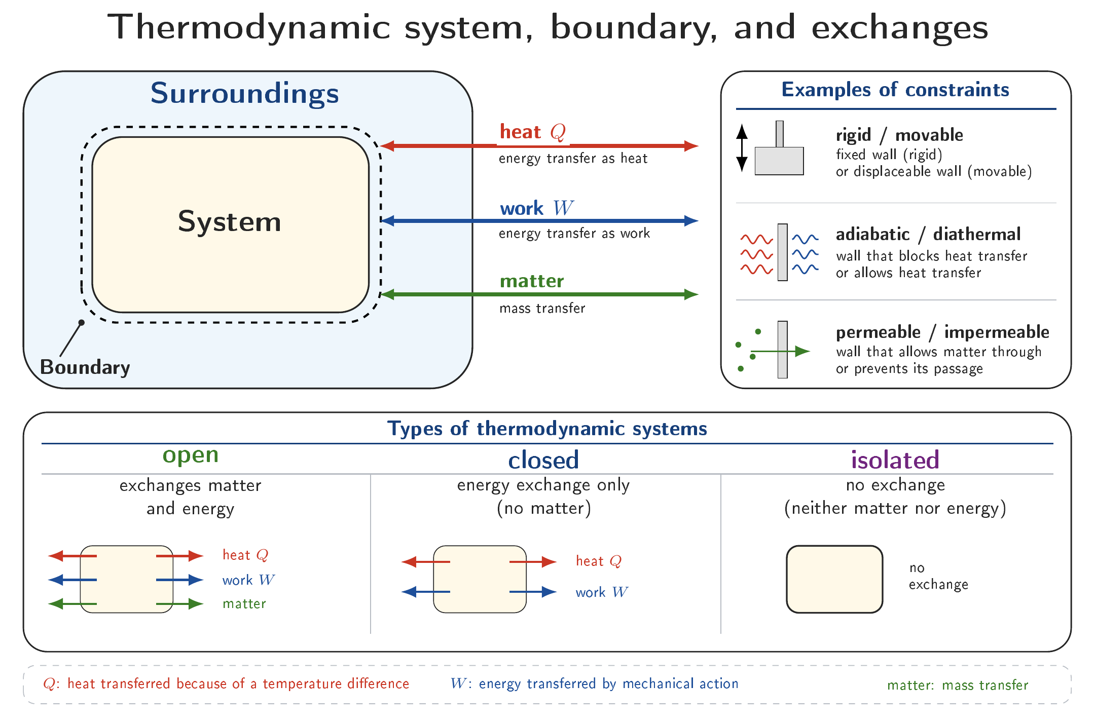
Once the system has been defined, the first question is what it can exchange with its surroundings. Two main kinds of exchange will occur in this course: exchanges of matter, and exchanges of energy, notably as heat or work. This leads us to distinguish three types of systems.

The fourth logical category—a system that exchanged matter but no energy with its surroundings—has no physical meaning: any matter crossing the boundary necessarily carries energy with it.

For example, a gas enclosed in a cylinder fitted with a piston is a closed system: no molecules cross its walls, but the gas can receive heat or do work by moving the piston.

An open pan of boiling water, by contrast, is an open system, since steam escapes from it and it can receive heat from the hotplate.

A perfectly isolated system is always an idealization. A sealed vacuum flask is a good approximation for a limited time. In reality, no system can be perfectly isolated, since even in a vacuum electromagnetic radiation can carry energy to or from the system; see Lesson 12 on radiation thermodynamics.

2. Boundaries, walls, and constraints

The properties of the boundary determine which exchanges are possible between the system and its surroundings. Different boundary conditions can produce entirely different thermodynamic evolutions from the same initial state.

In other words, knowing the system is not enough: we must also know the constraints imposed at its boundary. When a boundary consists of a material wall, several common cases are distinguished.

• A wall may be rigid or movable. A rigid wall fixes the geometry of the system. A movable wall, by contrast, can move under the action of unequal pressure forces on its two sides.
• A wall is called diathermal or diathermanous if it permits heat transfer, and adiabatic if it prevents it. One may also say thermally insulated, but adiabatic is more precise because it is not limited to thermal conduction: an adiabatic wall prevents every thermal energy transfer, whether by conduction, convection, or radiation.
• A wall may be permeable or impermeable to matter. It may also be semipermeable, meaning that it allows some chemical species to pass while blocking others.

Figure 1 summarizes the possible exchanges with the surroundings, the three types of systems, and the main constraints imposed by their boundaries.

These properties are constraints that determine which thermodynamic processes are possible. Consider, for example, two gases separated by a rigid wall. Their pressures may differ without anything happening because the wall prevents all motion. If the wall is replaced by a movable piston, the pressure difference sets the piston in motion.

Likewise, two bodies separated by an adiabatic wall may remain at different temperatures. If the wall becomes diathermal, however, heat is transferred until a new equilibrium is established.

Finally, two solutions containing the same chemical species at different concentrations can retain that difference when separated by a membrane impermeable to that species. If the membrane becomes permeable to it, the particles can cross the boundary and diffuse from one region to the other until a new equilibrium is established. In the simplest case, when the two media are otherwise equivalent, equilibrium corresponds to equal concentrations on both sides.

It is often useful to impose particular external conditions on a system without describing in detail the apparatus that produces them. For example, we may wish to study a system that is kept at constant temperature no matter what happens. In practice, it could be placed in an oven, a refrigerator, a water bath, and so on.

Formally, this amounts to imposing certain properties on the surroundings with which the system interacts. A reservoir is a system large enough that some of its parameters can be treated as constant despite exchanges with the system under study.

A thermal reservoir, or thermostat, is a reservoir whose temperature remains practically constant when it receives or releases a reasonable amount of heat. If a small body is immersed in a large lake, for example, the lake can be regarded to an excellent approximation as a thermostat.

Similarly, in many situations the atmosphere can be regarded as a mechanical reservoir that imposes an approximately constant pressure. It is then sometimes called a pressure reservoir. This will often be the case in exercises.

Later, we will also encounter particle reservoirs capable of imposing a chemical potential.

3. Thermodynamic equilibrium

Equilibrium lies at the heart of classical thermodynamics. The theory we are about to develop primarily describes equilibrium states and processes connecting such states.

The concept is phenomenological in origin. Experience shows that a system subject to fixed external conditions generally tends, after some time, toward a state in which no macroscopic evolution can be observed.

Consider, for example, a metal cube that has been left in a room for a long time. Its temperature no longer changes by a macroscopically observable amount. Now place the cube in a hot oven. The conditions imposed at its boundary have changed, and the system begins to evolve again: its temperature gradually increases. After some time this evolution ceases once more, and a new stable state is reached.

The system is said to have relaxed to a new equilibrium state. The time needed to reach this state, called the relaxation time, depends on the system and on the physical processes involved. It may be very short in some cases and very long in others.

This observation leads to the following definition.

Thermodynamic equilibrium therefore does not mean that every temperature, pressure, or concentration difference has necessarily disappeared. It means that no spontaneous macroscopic evolution is possible given the constraints imposed on the system. We have already encountered an example: two volumes of gas at different pressures, separated by a rigid wall, may form an equilibrium state under that constraint.

An equilibrium state is thus always defined relative to the constraints imposed on the system. If one of these constraints is removed, the state may immediately cease to be an equilibrium state for the new thermodynamic problem. The second law will later provide a general formulation of this tendency toward equilibrium and will allow equilibrium states to be characterized.

Finally, an equilibrium state must be distinguished from a steady state. In a steady state, macroscopic quantities no longer depend on time, but persistent fluxes may nevertheless remain.

The standard example is a metal bar whose ends are maintained at different temperatures. After some time, the temperature profile in the bar no longer depends on time, yet a continuous heat flux passes through it from the hot end to the cold end. The system is not in equilibrium; this is why the definition of equilibrium also requires the absence of macroscopic fluxes. Examples of macroscopic fluxes include flows of heat and matter.

4. Macroscopic states and state variables

The natural next question is how equilibrium states can be described quantitatively.

4.1. State variables

A macroscopic system contains an immense number of microscopic degrees of freedom. One litre of gas, for example, contains on the order of $10^{23}$ molecules. A complete mechanical description would in principle require the position and velocity of every one of them. Thermodynamics nevertheless assumes that, at equilibrium, this microscopic information can be replaced by a very small number of macroscopic quantities, called state variables because they characterize the macroscopic state.

The best-known examples are volume $V$, pressure $P$, temperature $T$, and particle number $N$. We will see that the first law introduces another, internal energy $U$, while the second law introduces yet another, entropy $S$. For the moment, we assume that these two quantities exist and characterize the macroscopic state of the system.

The remarkable nature of this postulate was emphasized in the general introduction. It is not usually made explicit in formulations of the first and second laws, yet it is clearly essential and logically precedes them. Temperature and pressure are not microscopic particle coordinates; they are emergent quantities that become relevant only on the macroscopic scale.

4.2. Extensive and intensive variables

These state variables fall into two broad categories.

Volume $V$, mass $m$, and particle number $N$ are examples of extensive quantities. In general, we will also assume that internal energy $U$ and entropy $S$ are extensive (see the remark below).

Temperature $T$, pressure $P$, and chemical potential $\mu$, by contrast, are intensive quantities. Chemical potential will be introduced later.

4.3. Algebra of extensivity

Extensive and intensive quantities obey a simple algebra. It is useful to formalize it by introducing homogeneous functions.

Extensive quantities are therefore homogeneous of degree $1$, whereas intensive quantities are homogeneous of degree $0$.

This definition immediately allows quantities to be combined. If $X$ is homogeneous of degree $k$ and $Y$ of degree $k'$, then $XY$ is homogeneous of degree $k+k'$, while $X/Y$ is homogeneous of degree $k-k'$.

For example, the ratio $V/N$ is homogeneous of degree $0$ and is therefore intensive: it is the volume per particle. Similarly, the particle density $N/V$ is intensive.

This property provides a way to check the consistency of a thermodynamic equation. Besides satisfying ordinary dimensional analysis, an equation must also be consistent with extensivity: both sides must transform in the same way when the size of the system is changed. Adding an extensive variable to an intensive one, for example, is meaningless. You should make a habit—indeed, a reflex—of checking this, at least for the final result of a calculation.

As an exercise, verify that the ideal-gas equation $PV = N k_{\mathrm B}T$ satisfies both constraints. Here $N$ is the number of particles. The relation can also be written in terms of the number of moles $n$, related to $N$ by $N=\mathcal N_A n$, where $\mathcal N_A$ is Avogadro's constant. Since $R=\mathcal N_A k_{\mathrm B}$, this gives the familiar form $PV=nRT$.

5. The space of equilibrium states

It is useful to give a simple mathematical formulation of what we have just postulated. Let $\mathcal E$ denote the set of equilibrium states accessible to the system under consideration. A state can be described by a finite number of independent variables

whose values determine it completely. The $x^i$ may represent temperature, pressure, volume, and so forth. These state variables then serve as coordinates on the space $\mathcal E$.

We have stipulated that these variables must be independent. Indeed, the various state variables of a system are generally linked by equations of state. The ideal-gas equation provides one example. We will clarify this point in the next section.

We will further assume that thermodynamic quantities depend smoothly enough on these coordinates for differential calculus to be used. In mathematical terms, the resulting model of $\mathcal E$ is a finite-dimensional differentiable manifold.

This formulation may seem abstract, but it merely makes explicit an assumption that many books use implicitly when they write quantities such as $dT$, $dV$, or $dP$ without further specifying the mathematical structure that makes them possible.

This geometrical construction will chiefly allow us to formulate the dependence among thermodynamic variables and the concept of a state function precisely, and to explain why the work and heat exchanged between an initial and a final state depend on the path followed, whereas changes in internal energy and entropy do not (see the following sections).

6. Equations of state

We have just modeled the set $\mathcal E$ of equilibrium states as a finite-dimensional manifold. We must now determine what fixes its dimension. Many state variables may be used to describe a system, but they are generally not all independent: relations connect some of them.

Consider an ideal gas. We saw in the preceding lesson that its equilibrium variables satisfy

For a fixed amount of substance $n$, knowing $V$ and $T$ is therefore enough to determine $P$, since $P=nRT/V$. The three quantities $P$, $V$, and $T$ are all state variables, but only two of them can be chosen independently.

The ideal-gas equation thus corresponds to

An equation of state therefore reduces the number of variables that can be chosen freely. For a closed ideal-gas system, for example, the number of moles $n$ is fixed, and the equation $PV=nRT$ defines a surface in the abstract coordinate space $(P,V,T)$. In this case, the physical space of equilibrium states of the ideal gas consequently has dimension $2$, not dimension $3$.

One may choose $(V,T)$ as coordinates on this space, but other choices such as $(P,T)$ or $(P,V)$ are possible. None is more physical than another: they are simply different coordinate systems on the same space of equilibrium states.

More generally, if we begin with $q$ state variables related by $r$ independent relations, only $d=q-r$ of them can be chosen freely. This number $d$ is precisely the dimension of the manifold $\mathcal E$. We will later see how to perform this count systematically.

7. State functions

Once the state space has been defined, we can introduce a concept that will be used continually.

If independent coordinates $x^1,...,x^d$ are chosen on $\mathcal E$, we may write $f=f(x^1,...,x^d)$.

Internal energy $U$ and entropy $S$ will be the two most important state functions in thermodynamics.

The differential of a state function is written

Between two equilibrium states $A$ and $B$, its change is

If $A$ and $B$ can be connected by a mathematical path $\gamma$ in the state space $\mathcal E$, then

This equality holds for every path $\gamma$ connecting $A$ to $B$: the integral is therefore independent of the chosen path. We say that $df$ is an exact differential. The path $\gamma$ introduced here is a mathematical object and does not necessarily represent the system's actual physical evolution. The next section specifies when a thermodynamic process can itself be represented by a path in $\mathcal E$.

This property will distinguish internal energy from heat and work. Heat and work are not quantities contained in the system; they are transfers of energy that occur during a process.

Their values therefore depend on how the process is carried out between its initial and final states. We will consequently write

for the elementary amounts of heat and work received by the system, to distinguish them from exact differentials of state functions such as

The symbol $\delta$ indicates that $\delta Q$ and $\delta W$ are not differentials of state functions. Heat and work will be defined precisely in Lesson 4, and entropy in Lesson 6.

8. Thermodynamic processes

A thermodynamic process is any process in which a system passes from an initial equilibrium state to a final equilibrium state.

During the process, the system is not necessarily in equilibrium. Its temperature or pressure may, for example, vary from point to point or even fail to be defined at all.

It would therefore be incorrect to represent the entire evolution by a path in the space $\mathcal E$ of equilibrium states. Only the initial and final states necessarily belong to this space.

8.1. Quasistatic processes

One class of processes plays a central role in thermodynamics: quasistatic processes.

In concrete terms, this means that the external constraints are changed sufficiently slowly compared with the characteristic relaxation times of the system.

All along the path, the system can then be regarded as passing through a succession of infinitesimally close states

and we may write

for example,

The quasistatic character of the process makes it possible to apply differential calculus throughout its evolution. State variables and all state functions are then defined at every stage, and their infinitesimal changes can be evaluated along the path followed in $\mathcal E$.

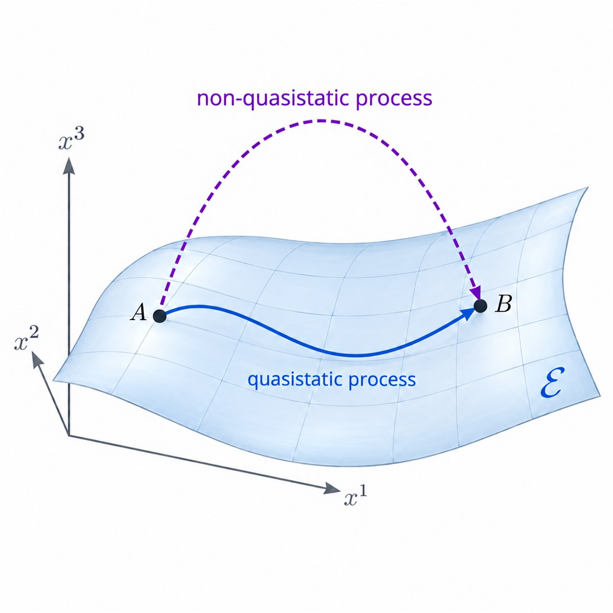
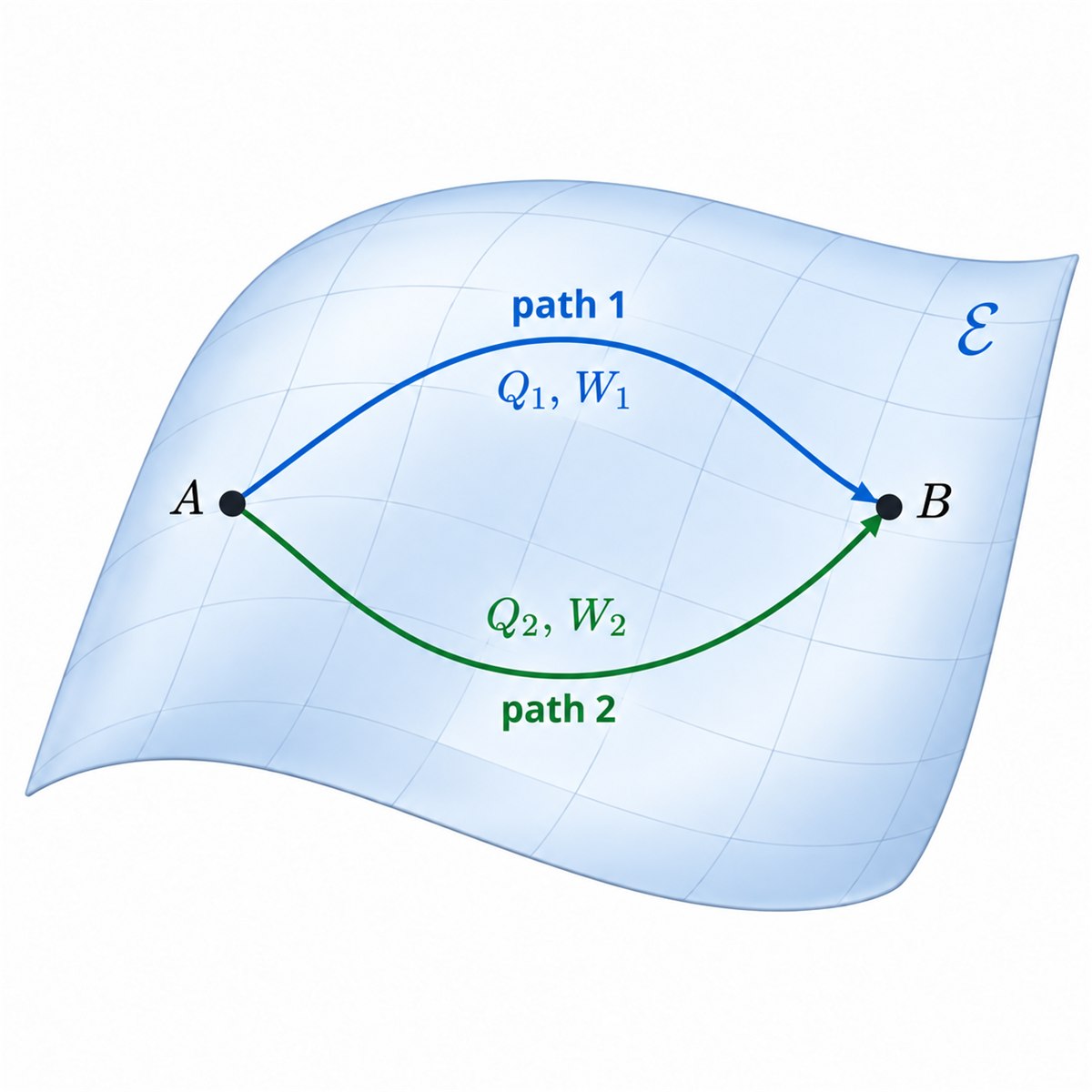
Figures 2 and 3 illustrate two aspects of this construction. The first contrasts a quasistatic process, which follows a path in $\mathcal E$, with a non-quasistatic process (for example, a sudden one), whose intermediate states are not necessarily equilibrium states. The second compares two quasistatic processes following different paths between the same states $A$ and $B$: the change in a state function is the same along both paths, whereas the heat and work exchanged may differ.

8.2. Special processes

Certain processes occur repeatedly in thermodynamics and are therefore given special names. When a definition concerns a property of the system, it assumes that this property is defined throughout the process.

• A process in which the system is in contact with surroundings at a constant temperature, $T_{\rm ext}=\mathrm{const}$, is monothermal.
• A process in which the system is subjected to a constant external pressure, $P_{\rm ext}=\mathrm{const}$, is monobaric.
• A process in which the system's temperature remains constant, $T_{\rm sys}=\mathrm{const}$, is isothermal.
• A process in which the system's pressure remains constant, $P_{\rm sys}=\mathrm{const}$, is isobaric.
• A process at constant volume, $V=\mathrm{const}$, is isochoric. This is notably the case for a system contained in a rigid vessel.
• A process with no heat exchange, $\delta Q=0$ throughout the process, is adiabatic. Ideally, it may be produced using adiabatic walls.
• A process at constant entropy, $dS=0$ throughout the process, is isentropic. In particular, it satisfies $\Delta S=0$ between its initial and final states. An adiabatic process is not necessarily isentropic, as we will see later.
• A process at constant internal energy, $dU=0$ throughout the process, is isoenergetic. In particular, it satisfies $\Delta U=0$ between its initial and final states.
• A process whose final state is identical to its initial state is cyclic.

Note that a monothermal process is isothermal under the condition of thermal equilibrium: if the system remains in thermal equilibrium with its surroundings at every instant, through a diathermal wall, then $T_{\rm sys}=T_{\rm ext}$ throughout the process. Likewise, a movable wall that allows mechanical equilibrium makes a monobaric process isobaric.

9. References

For a classical and systematic presentation of thermodynamics, see in particular Diu et al. ^[1] and Callen ^[2].